
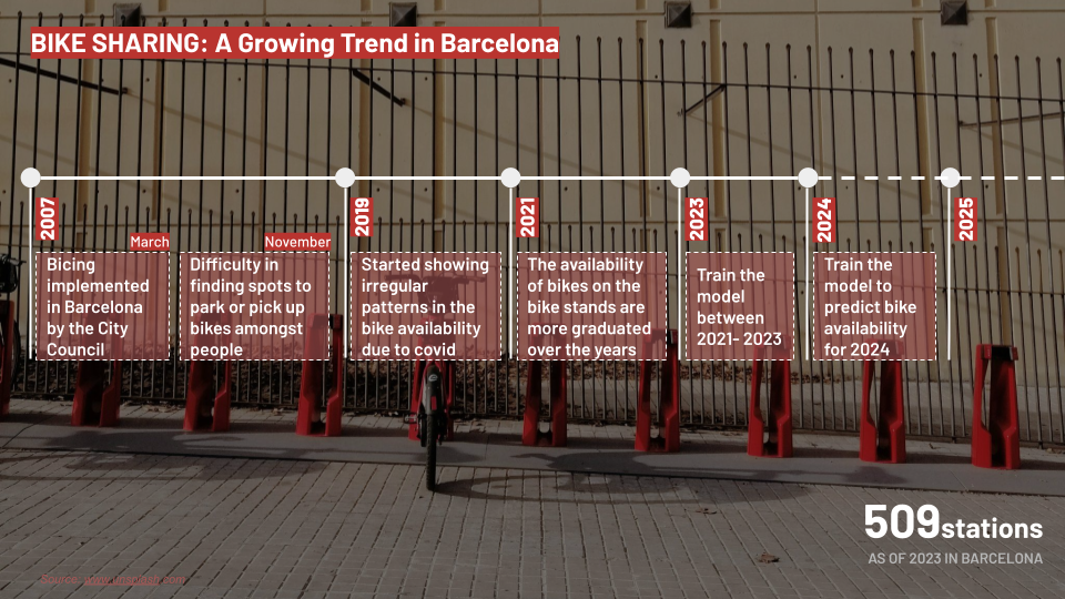
Bicing was launched in 2007 as a viable eco-friendly alternative or complement to traditional private and public transportation. The mobility network has also allowed for increased physical activity and better connectivity between neighbourhoods of Barcelona. It is aimed at anyone with a NIE, over the age of 16. The Bicing 2.0 models were released in 2019 to include electrical charging docks. Currently, ‘Smou’ is the mobile interface for Barcelona’s mobility sharing. The forecast for availability of bicycles is limited to a future prediction within the next 15-30 minutes.
The task of this project was to predict the availability of Bicing bikes at any given station in Barcelona at any given time during the first three months of 2024, using machine learning algorithms in Python.
Availability
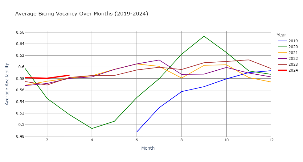
We started our investigation by looking at how the availability had varied over time in the period 2019-2023.
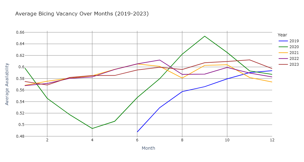
The graph shows that the availability pattern deviated from the typical behaviour in the first two years 2019 and 2020. This can be attributed to a number of causes. Firstly, 2019 was the year that Bicing 2019 was introduced, together with a new app. The app initially had many flaws, leading people to avoid the use of Bicing. The second dip, in 2020, was caused by the covid pandemic and the ensuing lockdown. Once the lockdown was lifted, Barcelona citizens wanted to avoid the tight spaces associated with public transport (bus, metro etc) and therefore chose Bicing instead. This explains the peak in August to October of 2020. As a consequence of this analysis, we decided to limit the training data of our machine learning model to the years 2021-2023.
Training data
To train our model we chose to rely on a number of different types of data:
- Spatial data – Latitude, Longitude, Altitude
- Temporal data – Month, Day (working day or not?), Hour of the day
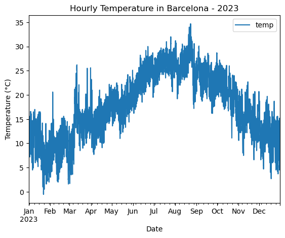
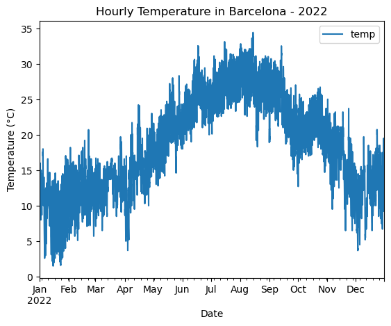
- Weather – Temperature
- Supply and Demand – population density, station capacity
The spatial data and temporal data were retrieved from or produced from datasets that were given as a default in the competition. Hourly temperature data was downloaded from the Meteostat python library.
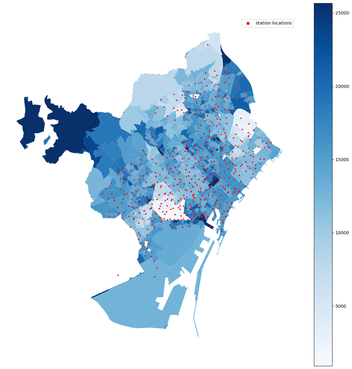
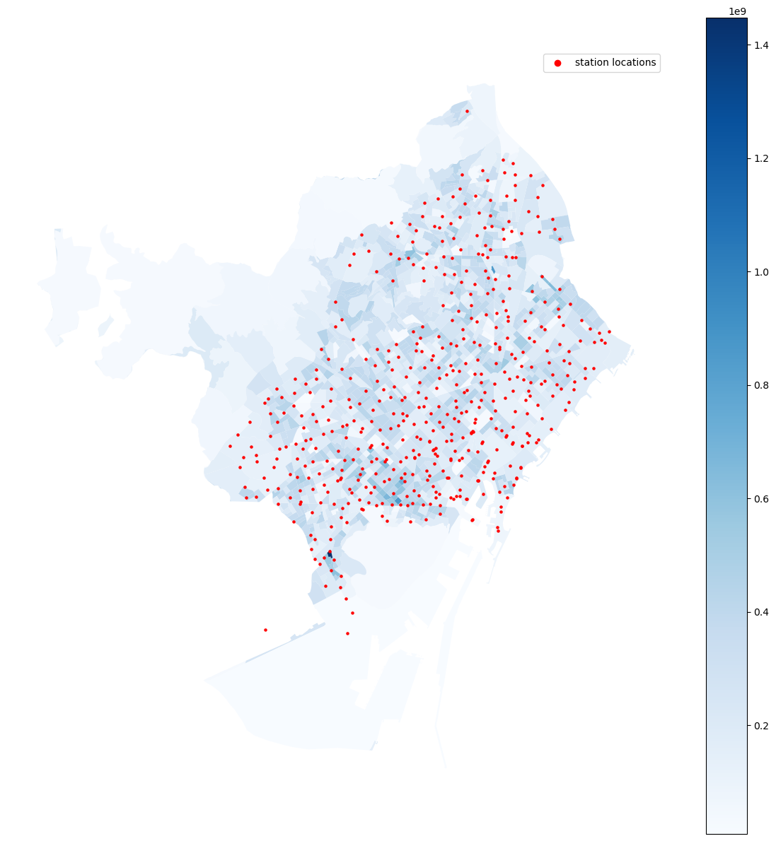
Population data was downloaded by censal neighbourhood from the Barcelona census. We then divided the the number by the area of those neighbourhood to calculate the population density. The maps below of (1) the absolute population numbers and (2) the population by area show that this important to get a correct understanding of expected us:
Training models
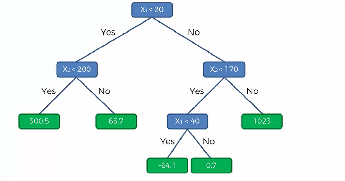
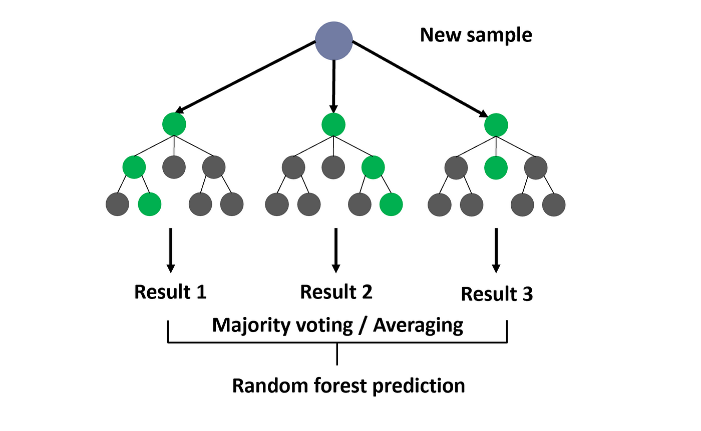
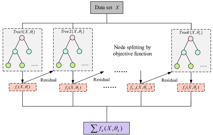
We experimented with three different machine learning models, all based on the principal of the decision tree (1). A decision tree builds a prediction by dividing the dataset into halves in several iterations, based on logical patterns in the numerical values of the training data. Once the model has been constructed it is possible to run a new set of data, lacking the predicted value (in our case availability), and through the model predict the value based of the other correlated data. A random forest (2) builds several decision trees and calculated the average prediction. A gradient booster regression (3) functions in a similar way, but in addition runs an an iterative process while training where every decision tree will try to improve based on success in predictions of the predecessor.
Result and lessons learned
The mean squared error for the three predictors was calculated to 0.064 for our decision tree, 0.023 for the random forest and 0.057 for the gradient booster. However, when compared to the actual data from 2024, we found that the best prediction was the gradient booster at 0.074. This means that all of our models were overfitted and therefore gave an illusion of predictive precision. Bellow we plotted our best prediction in relation to the existing training data.
During the presentations of our peers, we learned that our prediction could have improved by being more methodical in our approach in two ways:
Firstly we should have asked the question: Why are we using the data that we are using? Getting an understanding for the correlation between our chosen datasets and the availability parameter would have allowed us to select data with a high predictive power. In our case it seems like some of the data we added did not improve our prediction and instead added noise. Concretely it would have been important to have a good understanding the behaviour of availability in relation to the spatial, temporal, weather and supply/demand datasets that we chose in order to select the datasets that really mattered for the prediction.
Secondly it would have been important to motivate the choice of model based of training data. We learned from our peers that the data displayed nonlinear patterns in availability over the time of the day. This would motivate the use of a decision tree as opposed to some variation of a linear regression.
