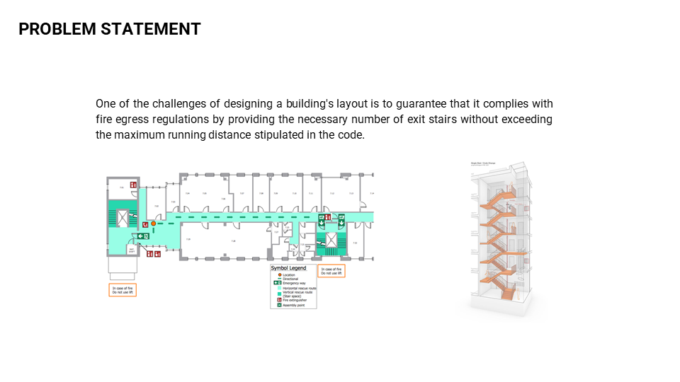
This initiative is oriented towards the practical undertaking of identifying egress points within a floor plan. We have analyzed three typologies of a structure akin to multi-family dwellings or hotel-style establishments. After a thorough engagement with the process, there are subsequent measures to be considered, which we intend to elaborate upon in our final review.
As an architect embarks upon the task of designing a floor layout, their accumulated expertise often provides an instinctive understanding of the optimal positioning for the egress points. Nonetheless, during the early design stages, adaptability and openness to innovation remain crucial. This is the juncture at which our project integrates with the design process.
Our initiative not only supports experienced architects but also serves as an invaluable tool for less experienced staff. By providing recommendations on the optimal placement of egress points during the floor plan design process, our tool aids junior architects when they are charged with producing floor plan alternatives. Consequently, this enables a transfer or codification of knowledge into the software’s programming, effectively facilitating intergenerational knowledge transfer within the architectural field.

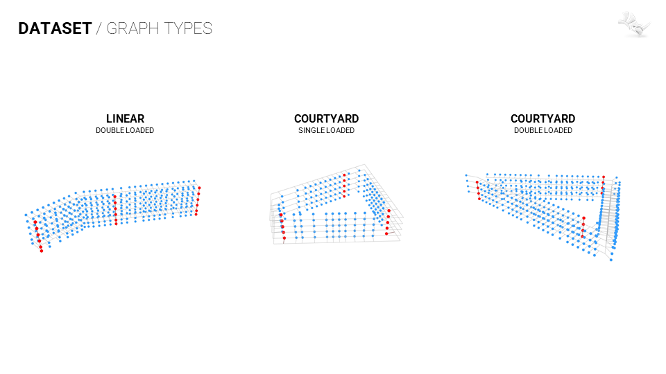
Below, the GIF represents the process developed within Rhinoceros/Grasshopper to develop the graph network.
- Take large rectangular boundary
- Populate within boundary with set number of points
- Cull points to the number needed for the typology
- Join points to create corridor center line
- Offset center-line for corridor walls and exterior walls
- Join exterior curves
- Trim demising wall lines and selectively remove some for room size variance
- In the training data, egress location is selected to maximize distance below 60m per IBC
- Center of each room becomes a node
- Perpendicular edges join to the corridor at another node
- Nodes and Edges with some features exported to python via CSV
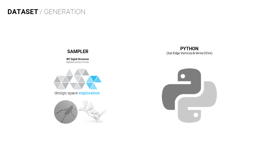
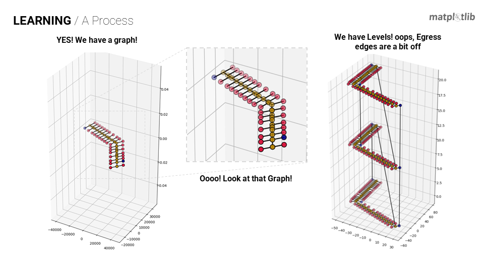
As the CSV files were brought into python the team created the graphs with the NetworkX library and visualized with matplotlib a charting and plotting python library. Each of the typologies were represented by 1000 iterations totaling 3000 input graphs.
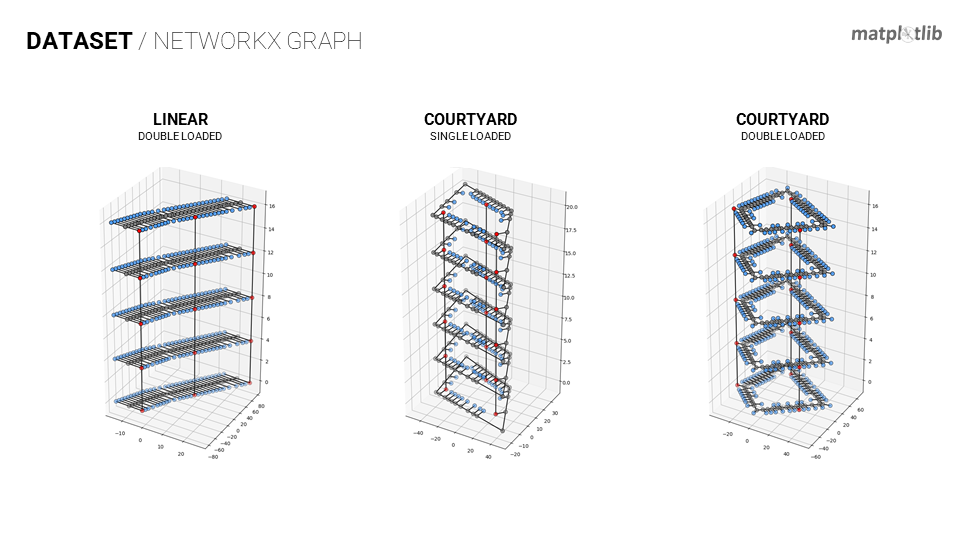
A GIF to show the variety of graphs that were produced to train our model.
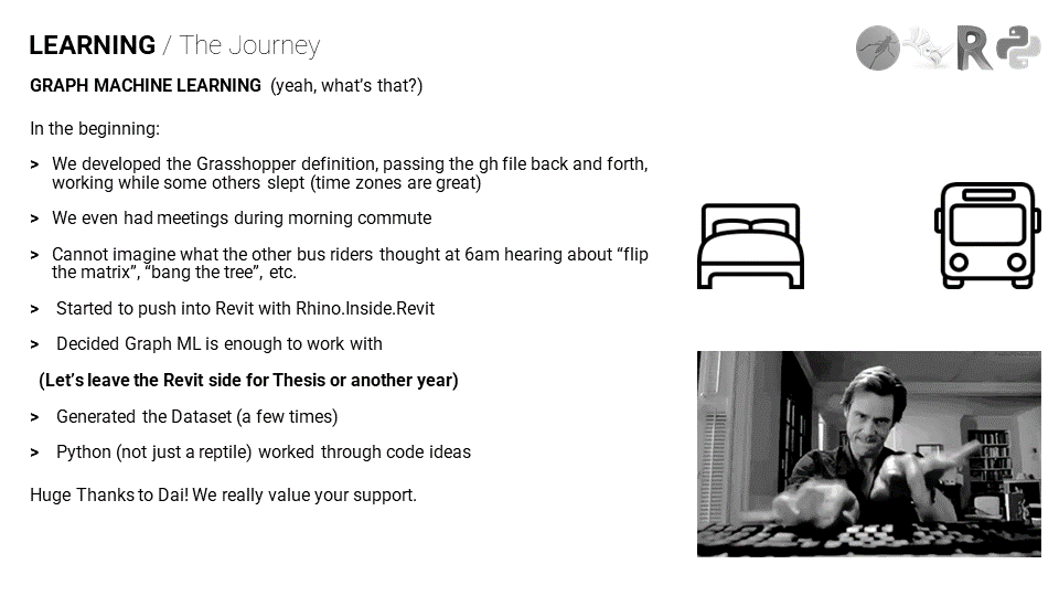
This third term of the MaCAD program has all been about process, of course a good output is wonderful. Machine Learning as a subject is vast and encompasses so much knowledge and experience. Our team worked well together, initially we would alternate working on the Grasshopper file. The time zone difference (12-16 hours) worked to our advantage as there would be some overlap hours of team members being awake then as some would be sleeping the others would be working. Therefore we were able to achieve more in less time which was key this term as it felt like the busiest term. We even held a meeting while one team member was commuting to work on the bus, imagine the other bus riders at 6am hearing “flip the matrix” and “bang the tree” along with the other commentary related to our gh definition. Our team considered pushing into Revit and the BIM realm, although we decided that Graph ML is enough in and of itself. Leaving the BIM side to Thesis or for another year to pick up and edge further.
We were very excited upon visualization within the Colab notebook environment. One floor’s graph was a good step and it looked great! Next step was going vertical, as can be seen the egress edges were not properly aligned and sorted prior to export of the CSV files. Back to the drawing board. Did we mention process was a big thing?
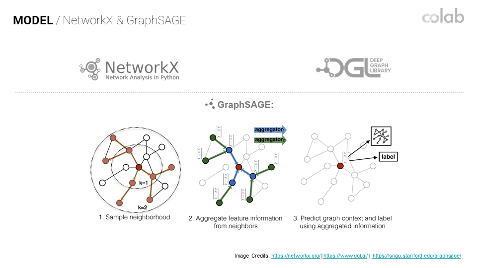
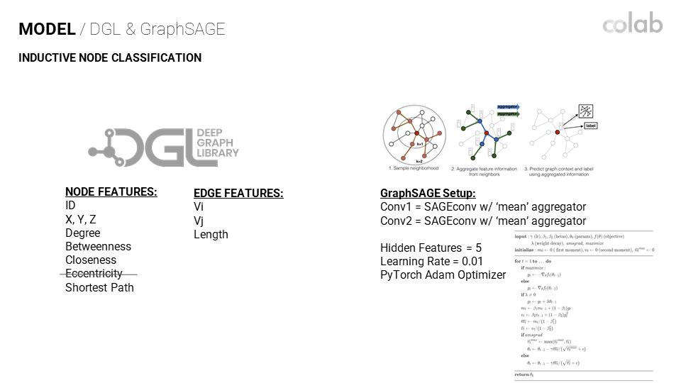
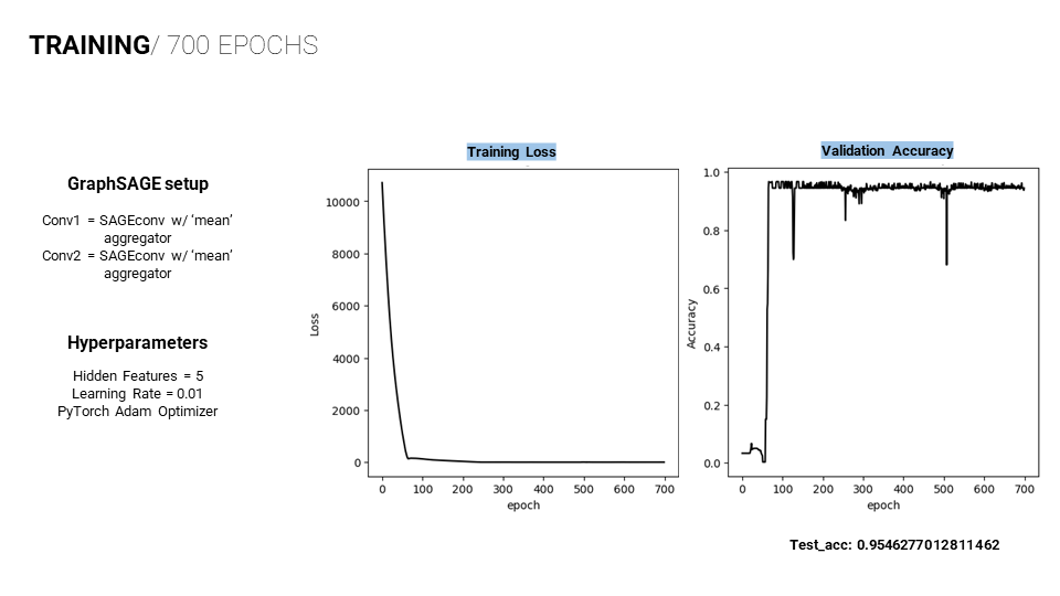
Once the data generation structure issue was settled the team could move forward with the graph training process. Within Google Collaboratory notebooks we were granted access to the NetworkX, Deep Graph Library (DGL) and GraphSAGE. NetworkX allowed us to convert the points and lines from Rhinoceros into the graph representation while DGL aided in the application of attributes. GraphSAGE was the chosen machine learning model for our Inductive Node Classification.
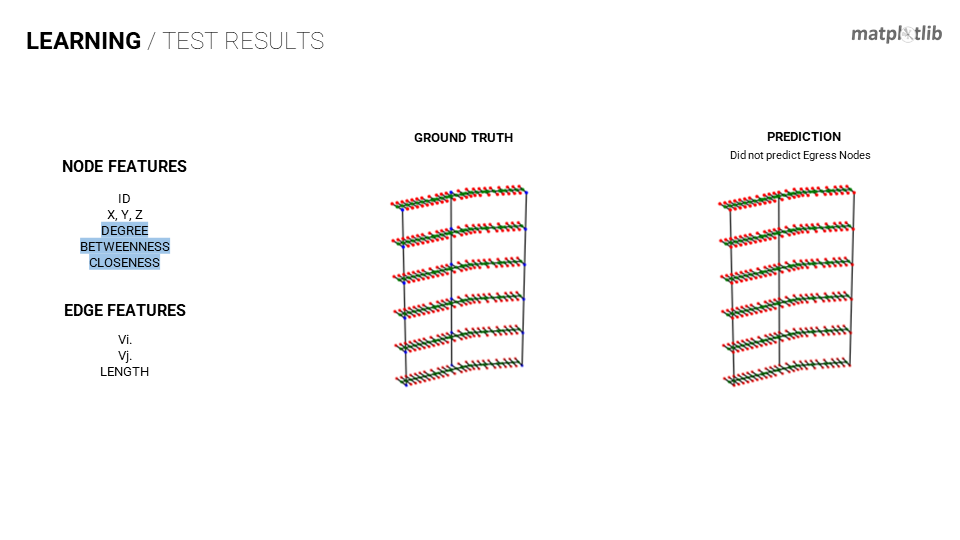
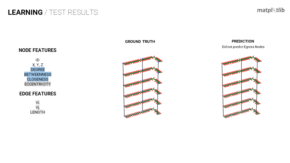
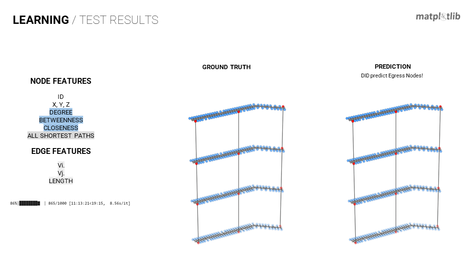
With DGL (Deep Graph Library) the nodes and edges had their features / attributes applied. Initially only the node’s ID, Coordinates, Degree, Betweenness and Closeness was applied. This was found to be inadequate for the model to learn what nodes should be egress nodes, it was able to predict the units and corridor nodes. With suggestion from our Faulty Assistant Dai, we tried the additional feature of eccentricity which is a metric of the node’s centrality in the whole graph. This also did not provide adequate information or difference to the model for egress node classification. The team had already been working with the shortest path methods within NetworkX although in an incorrect manner due to the nodes already being labeled. With a revision to the process the nodes could be determined thru the degree and all shortest paths. Thusly, our investigation landed on the correct use of shortest paths and the GraphSAGE model was able to learn where the egress nodes should be classified.
Only Degree, Betweenness and Closeness were not enough features to provide the required differentiation for inductive node classification.
Also, the addition of Eccentricity did not predict the egress node classification.
Finally, the addition of all shortest paths the model was able to learn and provide the egress node classification.
Training the model through 700 epochs showed a clear Training Loss plot while the overall test accuracy of 0.95 was also a healthy achievement. This model was saved and tested on unseen data, in which it succeeded with flying colors.
In conclusion the distillation of building information into graph format is an effective way to reduce complexity to present 3D architectural information in a way that machine learning algorithms are able to process. This is a step forward in a long journey to integrate AI and Machine Learning into the architectural practice and the design process specifically. There are many more avenues of investigation now that we know this is possible and have learned the tools available to get the job done. Onward to the next challenge.
Our team considered what our next steps would be in progressing this further. We decided that the vertical edges may have been a signal to the model for where the egress locations should be, moving forward we think another project could take it beyond. Where the longest shortest paths within the single floor plate are used to find the least amount of egress nodes that will service all unit nodes within the code stipulated maximum travel distance. This then would aid in additional edge creation to tie all the egress nodes from each level within the python environment instead of setting up that relationship in the training data specifically.