Never Miss A Ride

Introduction

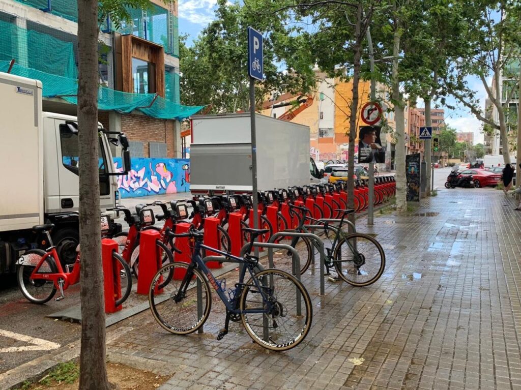
This presentation outlines the development and evaluation of machine learning models aimed at predicting the availability of bikes at various bicing stations in Barcelona. We’ll discuss the variables involved, the modeling techniques used, and compare the performance of different models.

Python is a friendly environment for preparing, training and forecasting machine learning algorithms within a variety of options and functionalities. For the specific need of this project, we focused on Regression models, for predicting numerical data, specifically focusing on Random Forests for managing data with no linear behaviour.

Initial Definitions

Data Exploration and Insights

We started with defining functions designed to manage and operate the pipeline, focusing on training, evaluating, saving and utilizing the models to make predictions. We first analyzed the competition-provided datasets to understand their structure and content.

The base input datasets included:

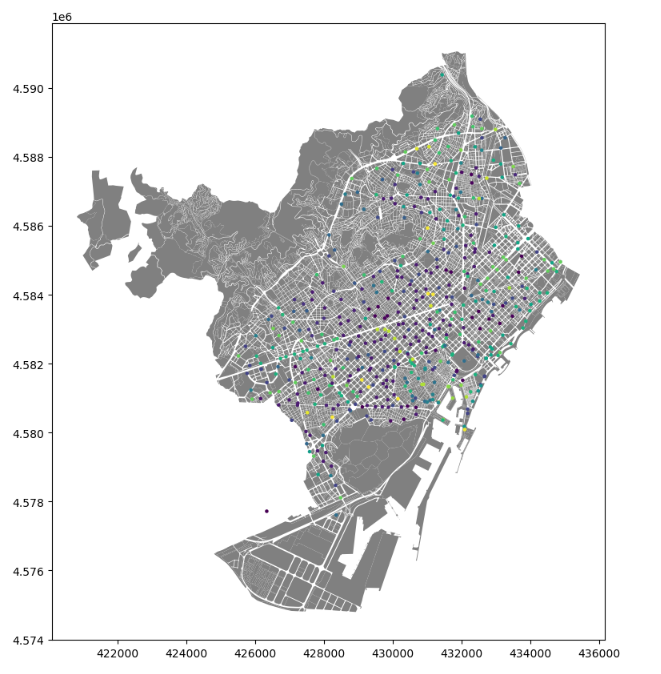
1. Characterization of Bicing stations in Barcelona, including their geographical position.
2. Time series of the hourly availability of each station from 2019 to 2023.

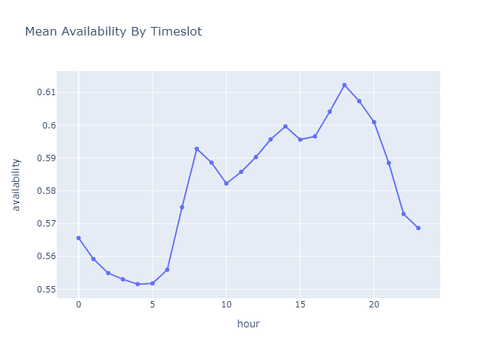
The exploration of the data informs a non linear behaviour that varies hourly, monthly or even yearly, highlighting the importance of implementing non-linear models for further training and prediction.

Further we understood the need for additional data to enhance our model, and explored and integrated relevant supplementary datasets. For this reason, we took into account variables related to weather, public transport accesibility, proximity to amenities, landuse, among others.

Each new dataset underwent thorough examination, cleaning, and pre processing before merging with our primary data, ensuring a robust foundation for our predictive modeling. Two specific indicators where used for removing invalid data:

1. Cases in which date was invalid (for example, the 31st of feburary)
2. Cases in which availability was not within a range from 0 to 100%

Training dataset

Exploring Historical Bicing Data

We began by examining the historical bicing data that was compiled and provided to us. As suggested by previous studies (Cenni, D., et al., 2021; Haw, A. et al., 2023) public bike availability at a given timeslot and date can be explained as a function of variables such as:

• Temperature
• Humidity
• Rain
• Pressure
• Wind speed
• Cloud cover
• Sunrise
• Sunset
• Availability in the same timeslot of the previous day
• Availability in the same timeslot of the previous week
• Socioeconomical variables
• Public transport accesibility

For this reason, to enhance our model’s accuracy, we explored incorporating data on station availability not only at the current moment but also from the previous day and the previous week.

This approach aimed to capture temporal trends and patterns in bike usage, which are crucial for accurate forecasting. By merging these time frames and calculating additional metrics such as bike occupancy and availability based on station capacity, our dataset was significantly enriched for more robust predictive analysis.

Adding Temporal Data for Events Over the Years of Study

Further, we expanded our data exploration by incorporating crucial temporal variables to enhance predictions on bike usage.

• Type of Day (Weekday, Weekend, Bussinessday, Holidays)
• COVID cases during lockdown

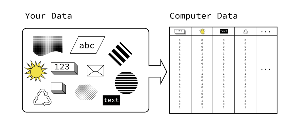
We created a time variable framework from our dataset, marking holidays and adjusting weekdays to identify business and non-business days. We applied One-Hot Encoding on weekdays to transform the categorical variables into a binary format, making them suitable for algorithmic processing.

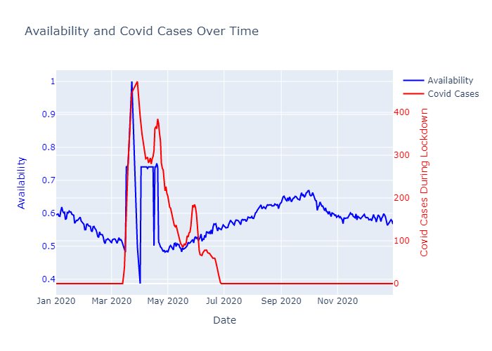
We also incorporated COVID-19 case data from Barcelona during the March 14 to June 21, 2020 (COVID Lockdown). This data was used to adjust for the expected decrease in bike usage during peak lockdown times, which helps prevent overfitting in our predictive models by ensuring the model does not learn anomalous patterns as normal.

Integrating Geospatial Data and Environmental Context

We further integrated other relevant datasets such as:

• Proximity to Public Transport : Joined to station ID as per the distance to nearest public transport node. (Source: OSM Data)
• Density of Local Amenities : Joined with station ID with a 300M buffer to quantify quality of access to amenities. (Soure: OSM Data, GTFS)
• Population Metrics : Joined with station ID as per total population in a 300M buffer. (Source: Census, 2018)
• Land Use Characteristics : Joined with station ID using a 25M buffer. (Source: Open Data BCN)
• Demand of Bicing by neighborhood in 2018 . (Bicing Demand 2018: . (Source: Pompeu Fabra University, 2018)

Environmental Data:

1. Weather Data : Joined with station ID by finding the nearest weather station. The weather dataset includes variables such as Precipitation, Wind Speed, Temperature, Humidity, Atmospheric Pressure (Source: Meteostat Python Library)

Comprehensive Pairwise Scatter Plot Matrices were used to visually explore correlations and distributions across multiple variables related to Bike Station Usage: Including Weather Conditions, Proximity Metrics, and Usage Statistics. These plots reveal patterns and outliers, facilitating deeper insights into factors affecting bike availability and utilization in urban settings. In this case, the plots showed non-evident correlation, again highlighting the non-linear behaviour of the data.

Creating PCA variables

Gathering independent variables makes the training dataset complex and might increase training and fitting times. For this, one approach that was assessed consisted in reducing the variables into Principal Components using the PCA technique, accross the following steps:

1. Standardise Data
2. Find New Dimensions
3. Select Important Dimensions
4. Reduce Complexity

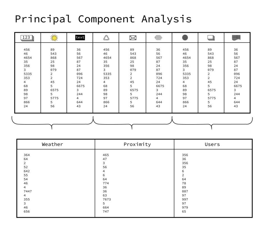
Through these approach, 6 latent variables were defined: i) Weather, ii) Proximity, iii) User Characteristics, iv) Time variables, v) Location and vi) Landuse.

Training models

We began our model experimentation by testing various regression models, ultimately identifying Random Forest as the most accurate and computationally efficient for our predictions. Although we also experimented with GradientBooster, Random Forest proved more suitable for our needs. Adjusting the estimator values in Random Forest to refine its structure revealed that higher values significantly increased memory usage and processing time.

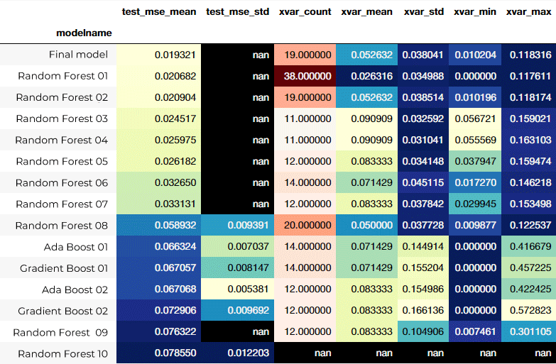
The different methods trained were assessed using the Mean Squared Error indicator, looking for the models that achieved lower error values. This analysis was also enriched with a Cross Validation. This means, training the model with different samples of the data (in this case using 75% of the dataset) and testing its performance with the 25% that remained.

The definitive model that showed the best performance is a Random Forest Regressor with 20 estimators and 19 variables including:

• Time variables: year, month, day, day of the week
• Weather: pressure, temperature, wind speed
• Station characteristics: capacity
• Proximity: to amenities, to metro stations, to bus stops

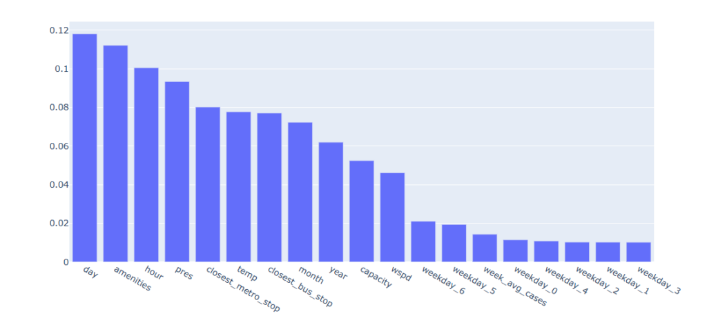
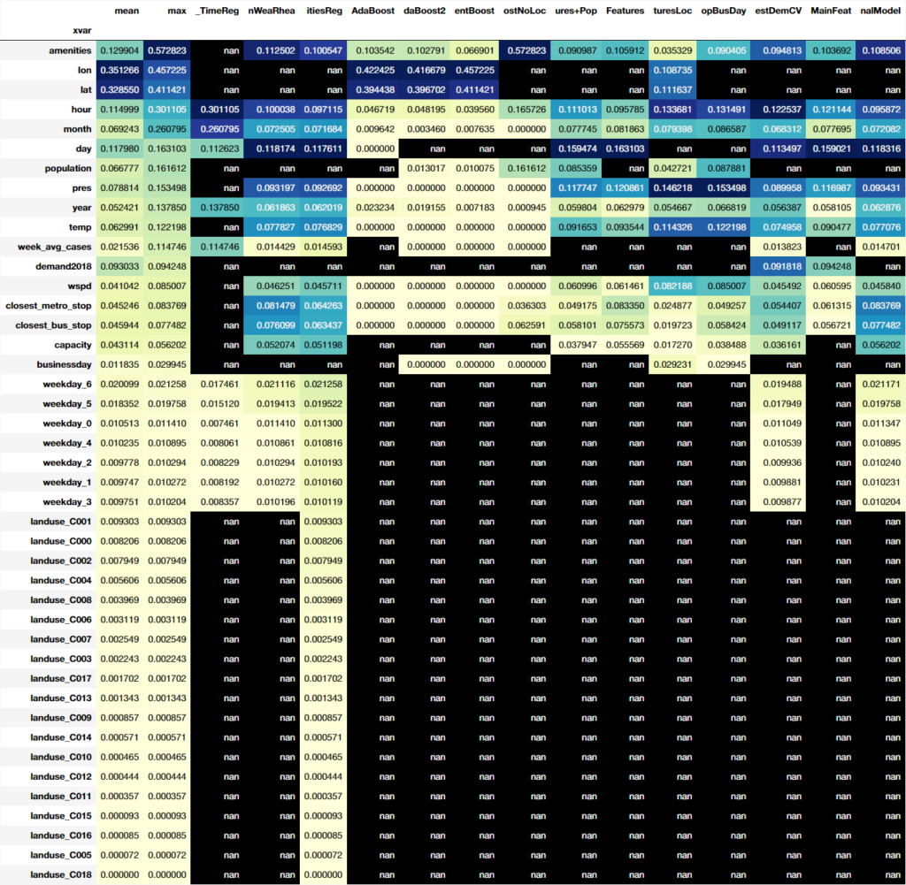
Finally, the performance of the models was also assessed through the measure of feature importance. The ideal model should output a balanced importance of all the features, avoiding few variables to take all the weight, or variables that don’t explain the behaviour of the dependent variable.

Feature importance in the definitive model

Prediction

The expected output is a prediction of the availability of each Bicing station for the 3 first months of 2024. Due to the nature of the variables assessed, two types of predictions methodologies were approached:

Full Prediction

This means running the entire model for prediction. This is the approach utilized for the definite model.

Recursive Prediction

For the cases where previous day or week availability was taking into account, the prediction needed to be recursive in cases where previous day or week data was not available in historical records meaning days in 2024. This model employs a recursive approach to predict day 1 availability and then uses this information to forecast availability for day 2, subsequently using these predictions to enhance future forecasts. Thus, the model continuously generates data on previous day or week availability, leveraging this to refine its predictions as it progresses.

Compare models

As explained above, we experimented with various models. Following are a few comparative graphs of some of the models we explored. When decribing the Mean Squared Error of the trained models, they showed an acceptable performance when training, reaching MSE values under 2%. When cross validation was implemented the error was higher but the dispersion of the error was less than 1%. Cross validation took high computation time and memory, reason why it could not be implemented in all of the models.

On another hand, assesing the feature importance, Proximity to amenities showed to have the maximum importance, followed by location variables. Nevertheless, the performance models did not include location variables.

Conclusions

The development of a variety of models showed the weight of including or excluding variables for achieving better performance. Nevertheless, although the training MSE reached values under 1%, the returned MSE of the predictions when compared to the actual historical availability in 2024 showed a MSE of over 6%. This means that the models are overfitting. Some strategies for future development of these models might include:

• Assessing less complex models and performing sensitivity analyses over the hyperparameters of the models
• Gathering socioeconomical data
• Identifying variables that might be producing high errors in specific clusters of the city

References

• Cenni, D., Collini., E, Nesi, P., Pantaleo, G., Paoli, I. Long-Term Prediction of Bikes Availability on Bike-Sharing Stations. Distributed Systems and Internet Technologies Lab, Department of Information Engineering, University of Florence. 2021
• Haw, A., Yeh, C. Zhuang, A. Predicting bike availability at bike share stations in Toronto. Bio-inspired Algorithms for Smart Mobility. Dr. Alaa Khamis, University of Toronto, 2023