
Catalonia is 50.6% forest. Within that territory, Aleppo Pine and Common Beech offer two contrasting structural profiles that can be processed with minimal industrial transformation — provided the right techniques are recovered and updated. This mid-term review documents the first half of our Studio II research into robotic steam-bending: a workflow that pairs a vernacular craft, the lofting tradition of Mediterranean boatbuilding, with robotic manipulation, treating each bent wood unit as an accumulator of elastic energy redirected into structural rigidity.
Wood as a local material
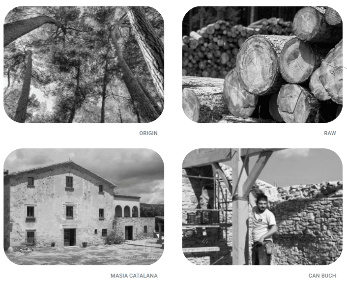
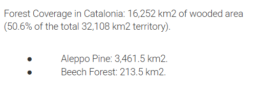
Catalonia is, despite appearances, a deeply forested region. 42% of its territory is wooded around 1.35 million hectares, making it the fourth-largest forest area in Europe after Finland, Sweden and Austria and roughly 75% of that surface is privately owned, with only a quarter under active management. The resource is abundant and underused.
Two species framed our research. Aleppo Pine (Pinus halepensis), locally pi blanc, is the most frequent forest type in the Catalan landscape, covering around 239,000 hectares, drought resistant, abundant, and structurally limited by its irregular grain. European Beech (Fagus sylvatica) is the opposite case: a smaller, wetter presence in the north, with the straight grain and long fibres that have made it the European reference for steam-bending since Thonet. Beech became our primary candidate; pine remained for lower-stress roles.
The masia, and Can Buch
The masia is the architectural answer Catalonia has given for centuries to the question of what to build with what is already there. A rural construction common across Catalonia, Valencia and southern France, built from stone, adobe and timber sourced within walking distance of the site, its structural intelligence comes from a precise reading of local material. The rehabilitation of Can Buch, a masia in Sant Aniol de Finestres (Girona) led by architect Oriol Roselló Viñas, brings that logic into the present. The project was documented as a demonstration that traditional techniques, using local materials handled by craftspeople, are a viable answer to today’s sustainability challenge.
Lofting and the mechanics of bending
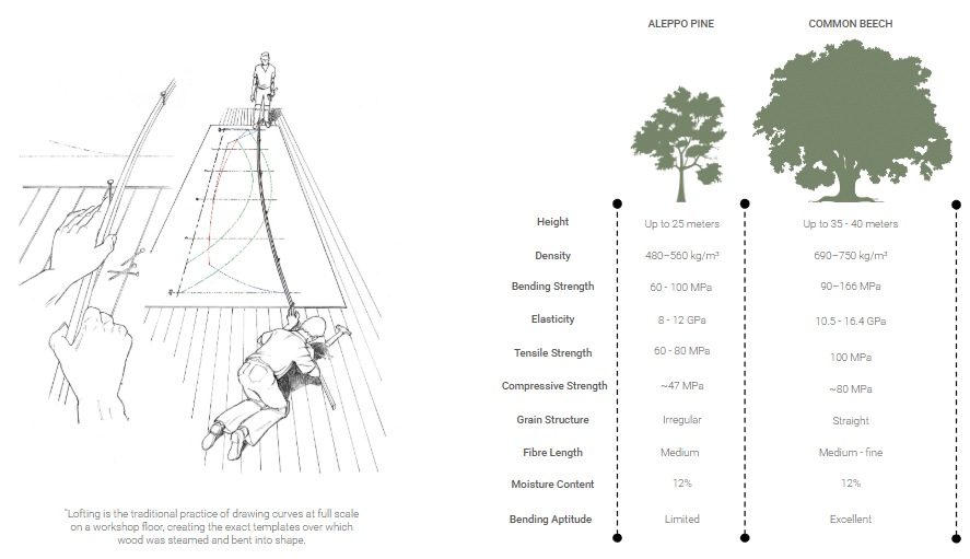
Before any wood is bent, the curve has to be drawn. Lofting is the practice of drawing full-scale curved lines and surfaces on a large flat surface, typically a dedicated loft floor, to generate accurate templates from smaller-scale plans. The term comes from the large lofts in shipyards where full-scale plans were traditionally drawn on the floor; in Mediterranean and Atlantic boatbuilding, the loftsman would lay out the hull’s lines at 1:1, fix flexible wooden battens against nails to pass through plotted points, and produce the templates over which steamed timber was bent into shape.
Lofting interests us for two reasons. First, because it externalises the geometry: the curve exists in physical space, at full scale, before the material is touched. Second, because it is inseparable from the bending process it serves.
Material properties
The mechanical comparison between the two species confirms the choice. Beech outperforms Aleppo Pine in every variable that matters for active-bending: roughly 50–65% higher bending strength (90–166 vs 60–100 MPa), ~30% higher modulus of elasticity (10.5–16.4 vs 8–12 GPa), and a straight grain against pine’s irregular one. Beech became the structural species; pine remained for secondary, lower-stress roles within the same system.
System logic
The proposal is structured as a chain of physical transformations:
Each bent strip is a battery of potential energy. Steam-bending introduces internal stresses — tension on the outer fibre, compression on the inner — that do not disappear once the curve is fixed. Captured at the right moment, they become the mechanism holding the assembly together: flexible laths, individually weak, turn rigid when their stored elastic energy is constrained instead of released.
The second principle is planar contact logic. Strips meet on their flat faces, never edge-to-edge. This maximises contact surface at every joint, distributes interlaminar stress evenly, and produces high-friction connections without heavy hardware. Complex global geometry emerges from a single repeatable rule: bend the unit, lay it flat against the next, fix the contact.
Active bending supplies the force; planar contact channels it. The tension trying to spring the wood back is precisely what locks the system in place.
Methodology
The workflow is split into two phases — pre-treatment (steam and moisture conditioning) and material manipulation — with manipulation tested at two levels of agency.
Manual manipulation
We began with bending boards and modular jigs: pegboards with reconfigurable pegs and clamps that act as physical control points for bending the conditioned strip. The goal was calibration — understanding how the material locks tension into a curve, how it releases on removal, and how moisture, radius, and dwell time interact. This stage exposed the spring-back effect directly, before introducing it into the digital pipeline, and produced our first working envelope: 4–5 min bending, 24 h drying, minimum radius ~70 mm, maximum ~310 mm, with PVA glue as primary fixing.
Robotic manipulation
The process then moved to a robotic arm, which grips one end of the strip and traces trajectories that pull the wood around fixed contact points — hitting radii that manual bending cannot guarantee consistently. Each piece is produced with 4 nodes, 2 movements, and ~2 minutes of robotic time.
What the robot adds is not force but repeatability and trajectory accuracy. The artisan’s intuition becomes a parametric trajectory, and the material’s elastic memory becomes a calculable variable rather than a felt one.
Pre-treatment
Predictable bending requires predictable material. We work with 4 mm strips of pine and beech (600 and 800 mm), soaked for up to 2 hours and steamed for a 12-minute cycle, with up to 5 minutes of steam exposure before manipulation. Target moisture content at bending is 28–32%, tracked with embedded MC sensors in both the strip and the steambox.
This gives a 5-minute working window before the wood hardens. Outside it, the strip either refuses the curve or fractures. Upstream MC control is the single most sensitive variable in the workflow — small deviations translate directly into geometric inconsistency downstream.
Robotic trajectories and unit geometry
With pre-treatment standardised, the next variable is the path the robot follows while bending each strip. The geometry of a unit is not defined only by its endpoints; it is defined by the trajectory the end-effector traces between them, the position and number of fixed contact points on the bending board, and the speed at which the curve is forced into the material.
The studies above map this design space.
The first set of trials, beginning with manual bending on the pegboard and translated to robot motion, calibrated the basic working envelope for beech: minimum radius ~70 mm, maximum radius ~310 mm, 4–5 minute bending window, and roughly 2 minutes of robotic time per piece, distributed across 4 nodes and 2 movements.
The second set explores multi-radius curves — pieces in which the radius changes along the length of the strip, producing units that combine tight and open curvatures within a single member. Each diagram annotates the radii (in mm) at successive segments. These compound curves are what allow a single unit to perform differently along its span: storing more energy where the curvature is tight, transitioning into smoother sections where it needs to meet another unit cleanly.
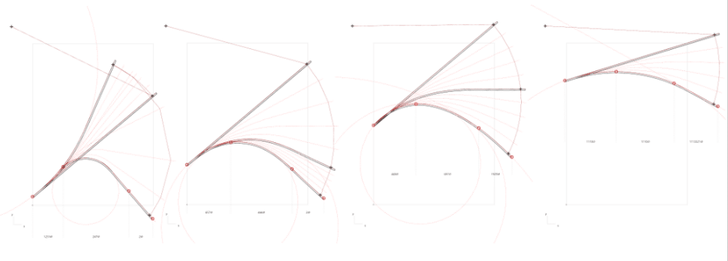
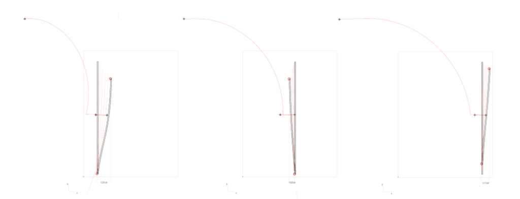
The third set tests the opposite extreme: large-radius, near-straight trajectories, where the strip is barely deformed and the robot traces long, shallow arcs. These low-stress units are candidates for the secondary roles — connection blocks, infill members — where pine becomes a viable species again.
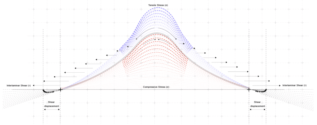
Forces: anatomy of bending stress
When a strip is bent, two opposing stress fields develop along its section. The outer fibre — the convex side of the curve — is stretched and works in tension (σ). The inner fibre — the concave side — is compressed and works in compression (σ). Both peak at the apex of the curve, where curvature is highest, and decay toward the supports.At the anchoring points, the stress field changes character. The strip wants to release its bent state by sliding along its length, generating interlaminar shear (τ) at the supports and a measurable shear displacement in the surrounding material. This is the force the connections must absorb: not a vertical load, but a longitudinal slip driven by the wood trying to straighten itself.
Connections
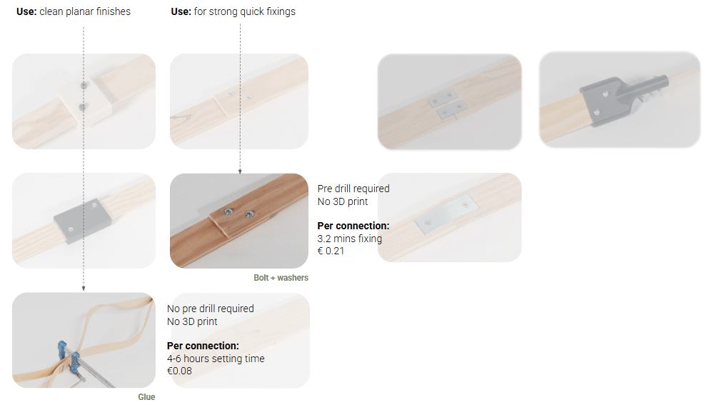
We split the catalogue into two families. Planar connections join strips along their flat faces, either overlapping or aligned. Non-planar connections join strips at angles through 3D-printed end fittings. Within the planar family we tested seven options — 3D-printed clamps, naked bolts, bolts with washers, screws, glue, and metal plates — and two advanced as the working pair:
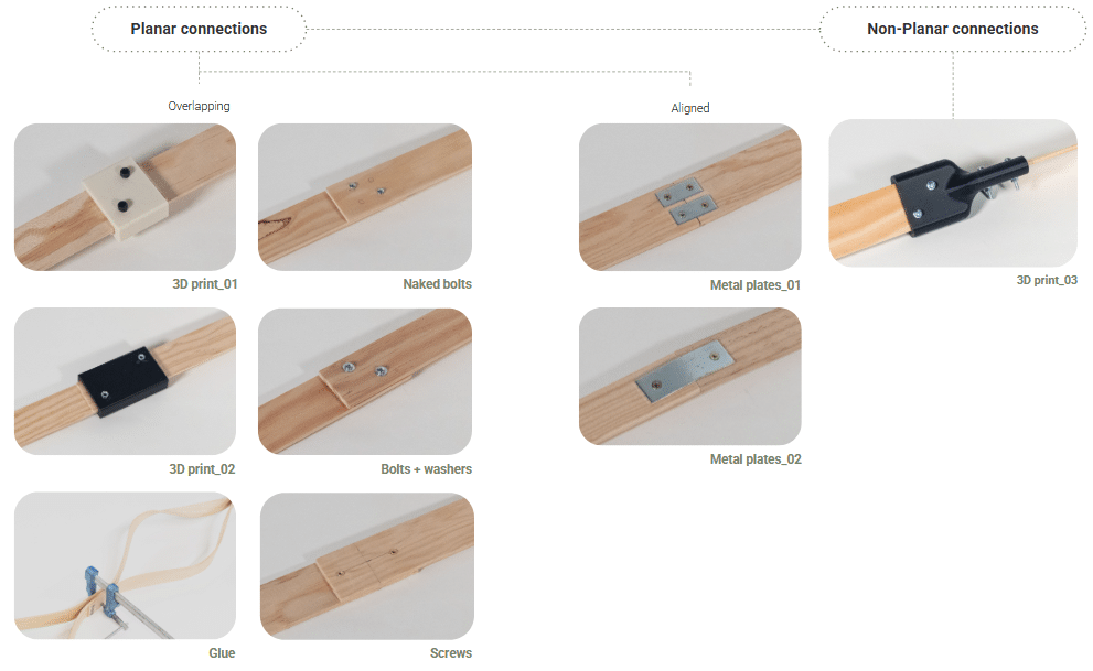
We keep both rather than choose. Glue is cheaper and cleaner but slow; bolts are forty times faster and resist shear directly through the fastener. They map onto the stress diagram: glue does the mid-curve, where tension and compression spread across large contact surfaces; bolts do the supports, where interlaminar shear concentrates and the joint has to resist slip.
Structural anatomy
The two solutions follow different rules.
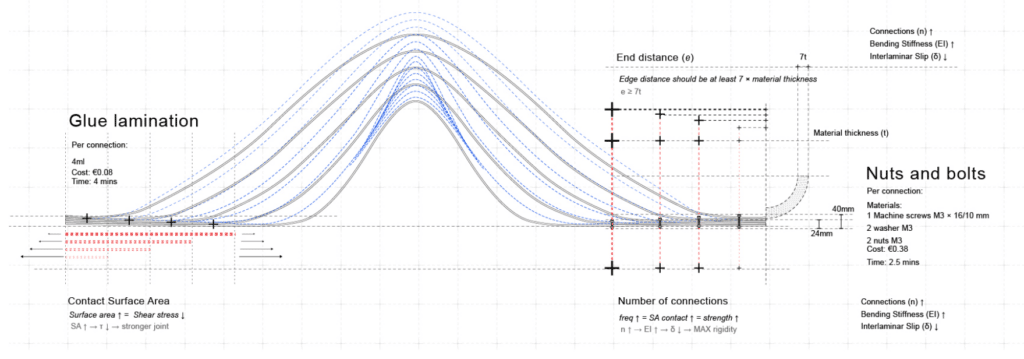
For glue lamination, the governing variable is contact surface area. The relationship is direct: as surface area increases, shear stress (τ) decreases, and the joint gets stronger. Per connection, glue uses 4 ml of PVA, costs €0.08, and takes 4 minutes of active work.
For bolts + washers, two variables govern. End distance must be at least 7 × material thickness (e ≥ 7t) to avoid splitting at the edge. And number of connections drives stiffness: more bolts → higher contact frequency → higher bending stiffness (EI), lower interlaminar slip (δ), maximum rigidity. Per connection: 1 M3 × 16/10 mm screw, 2 M3 washers, 2 M3 nuts, €0.38, 2.5 min.
Together the two rules close the loop: glue maximises rigidity by increasing surface, bolts maximise it by increasing frequency. Both translate the stress diagram into measurable design parameters.
Unit catalogue
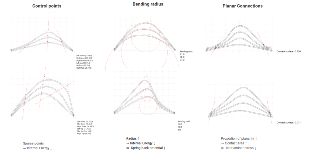
Each unit is defined by three parameters: control points (sparse → lower internal energy; dense → more locked tension), bending radius (large → less spring-back; tight → more stored force, closer to fracture), and planar connection proportion (high planarity → larger contact area → lower interlaminar stress). The two examples range from a contact surface of 0.226 down to 0.071.
The parameters are coupled — tighter radius stores more energy but fails earlier; high planarity strengthens the joint but constrains the geometry. The catalogue is the design space within those trade-offs.
Results
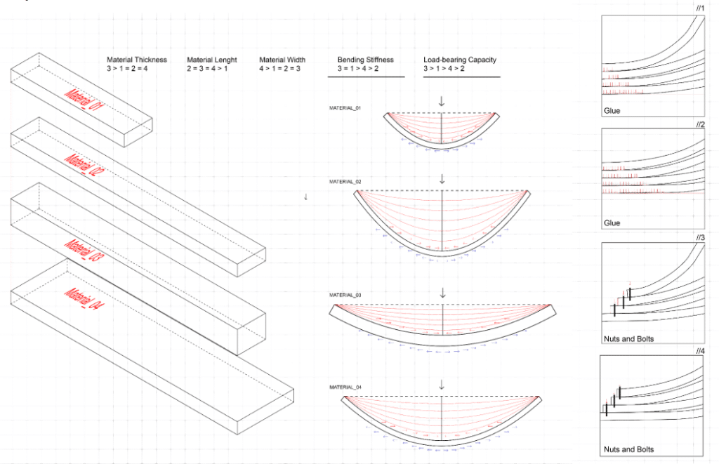
To validate the catalogue, four units were tested under load with different combinations of material thickness, length, and width, and ranked by bending stiffness and load-bearing capacity. The results map onto the connection logic from the previous section. Glue-laminated specimens (//1, //2) failed by separation along the contact surface — the joint released progressively as shear exceeded what the adhesive could distribute. Bolted specimens (//3, //4) failed locally at the fastener, with the surrounding wood remaining intact. Two findings carry forward into the next phase:
Failure mode is connection-driven, not material-driven. The wood holds; the joint releases. This confirms that the next iteration’s gains will come from refining the connection logic — not from changing species or thickening the strips.
Material thickness is the dominant variable for both stiffness and load capacity. Length and width matter, but section depth governs the curve.
From unit to system
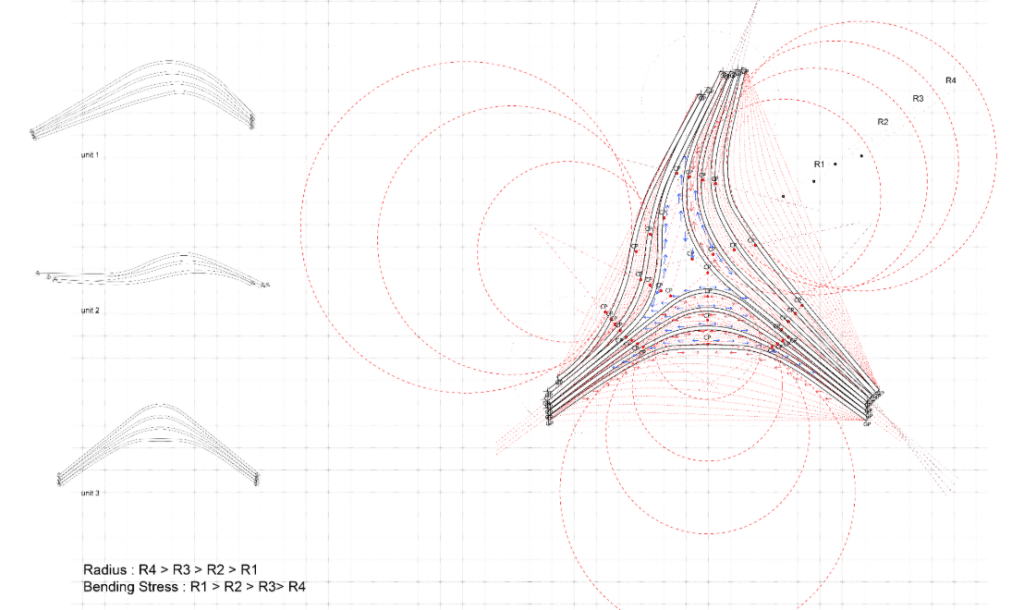
The individual units combine into modules by sharing gripping points. A module is the result of three or more units meeting at common anchors, with their bending radii distributed unevenly across the geometry: tighter radii (R1, R2) sit where the module needs to store more force; larger radii (R3, R4) sit where the geometry needs to relax. Bending stress and radius scale inversely — R1 > R2 > R3 > R4 in stored energy, R4 > R3 > R2 > R1 in radius — and arranging them deliberately is what gives each module its structural character.
The current module catalogue holds six configurations so far, each indexed by three variables: number of gripping points (3 or 4), curvature index (0.25–0.85), and central void area (minimum to maximum). We are still expanding it.

These modules then aggregate into a system matrix — a parametric structure where module behaviour is tuned to its position. Support zones use more slats, thicker sections, and shorter spans for greater strength. Higher levels use fewer slats, thinner sections, and longer spans for greater flexibility. The same geometric logic, scaled differently, performs as foundation or as canopy depending on where it sits.
Next steps
The second half of the term moves toward a 1:1 prototype of the system matrix. Three lines of work feed into it: characterising spring-back across radii, species, and moisture content so it becomes a controllable variable in the Grasshopper definition; refining robotic trajectories for compound and multi-radius curves; and pairing glue lamination with bolted joints across the same unit, following the stress logic established in the forces diagram.
