
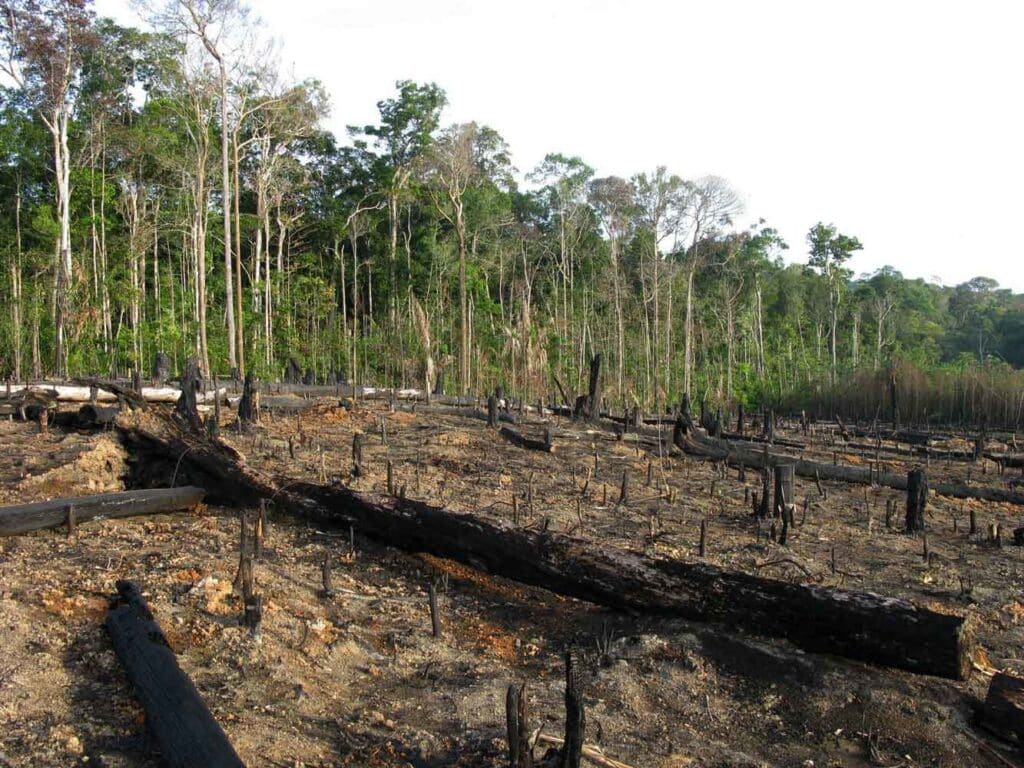
Timber is booming in architecture, often framed as a climate solution. But carbon is only part of the story. Forests are living systems whose shape matters: edges, cores, perforations, and bridges all affect biodiversity, microclimate, and resilience. Timber Trace asks: What does logging monitoring really tell us about the hidden impact of timber in architecture, and how do we bring that into early-stage decisions?
Timber Trace builds an AI-driven pipeline that segments forests from satellite imagery, isolates the clearings within them, and converts those shapes into standard landscape metrics. The result is a set of georeferenced, comparable indicators designers can read at a glance, which is patched into Rhino/Grasshopper for live iteration.
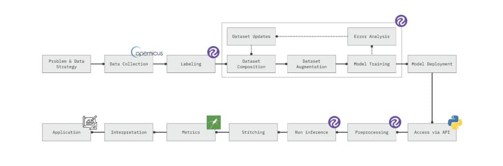
PIPELINE
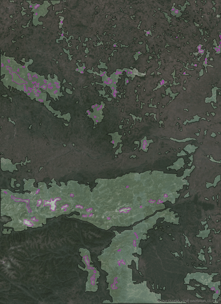
Imagery → Masks: Instance segmentation identifies forest patches and the non-forest fragments inside them (roads, cuts, clearings). The model is trained on tiled (64×64 px) scenes with SAM-assisted labeling and light augmentation. YOLOv11 powers instance segmentation.
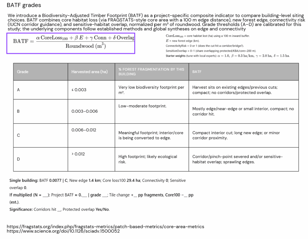
Masks → Metrics: From each patch the script computes patch density, forest area density (FAD), perimeter–area ratio (PARA), edge density, core share after inward buffers (100–200 m), largest connected component (LCC), and a corridor/bridge count (NSCP). These translate images into ecological meaning (fragmentation, edge exposure, and connectivity).
Live in CAD: Everything runs as georeferenced geometry and updates live in Grasshopper. This let’s you nudge a footprint or sourcing radius and instantly see the biodiversity implications.
ANALYSIS
The team is responsible for three Austrian sites that span the supply chain:
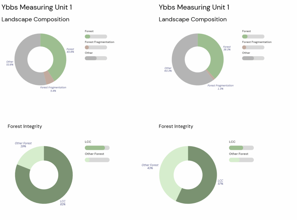
Ybbs an der Donau (Lower Austria, Austria): This site features river corridor logistics and a major Stora Enso sawmill surrounded by intensively managed mixed conifer forests, which are ideal for analysing harvest patterns and core-area loss.
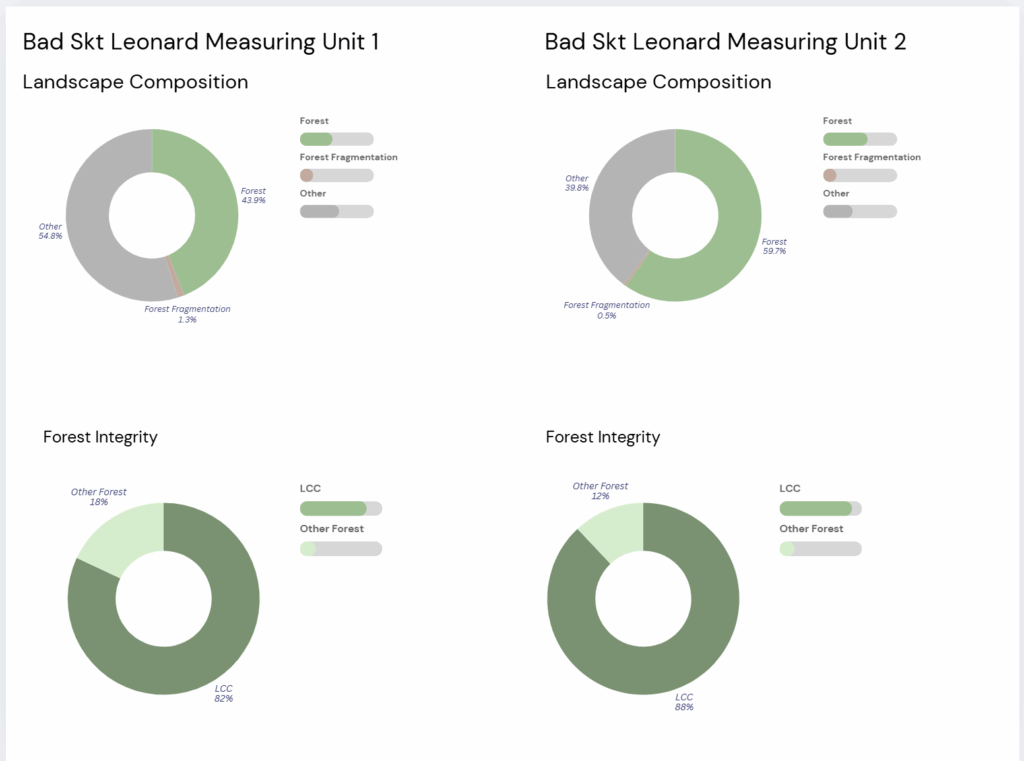
Bad Sankt Leonhard (Carinthia, Austria): An alpine valley dominated by spruce with frequent production and salvage cuts that create micro-fragmentation.
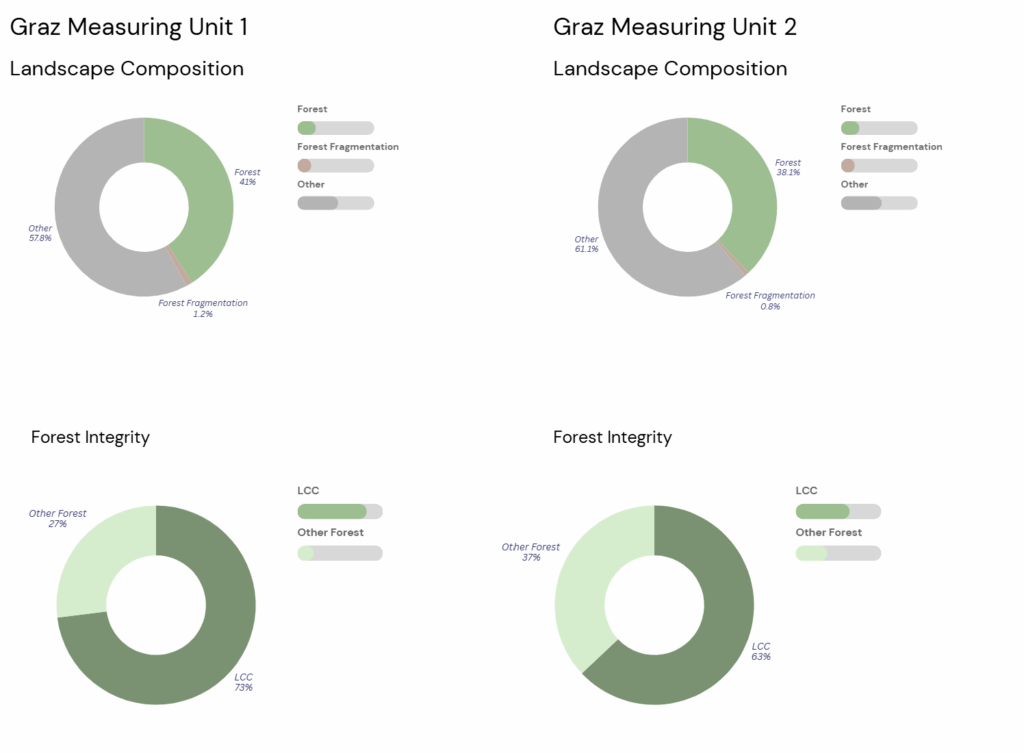
Graz (Styria, Austria): An urban demand centre near multiple harvesting districts, making it perfect for ‘urban timber boom’ scenarios.
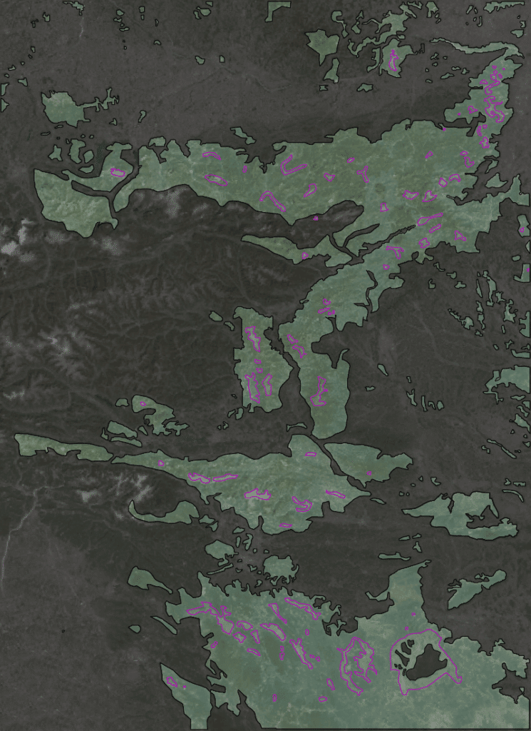
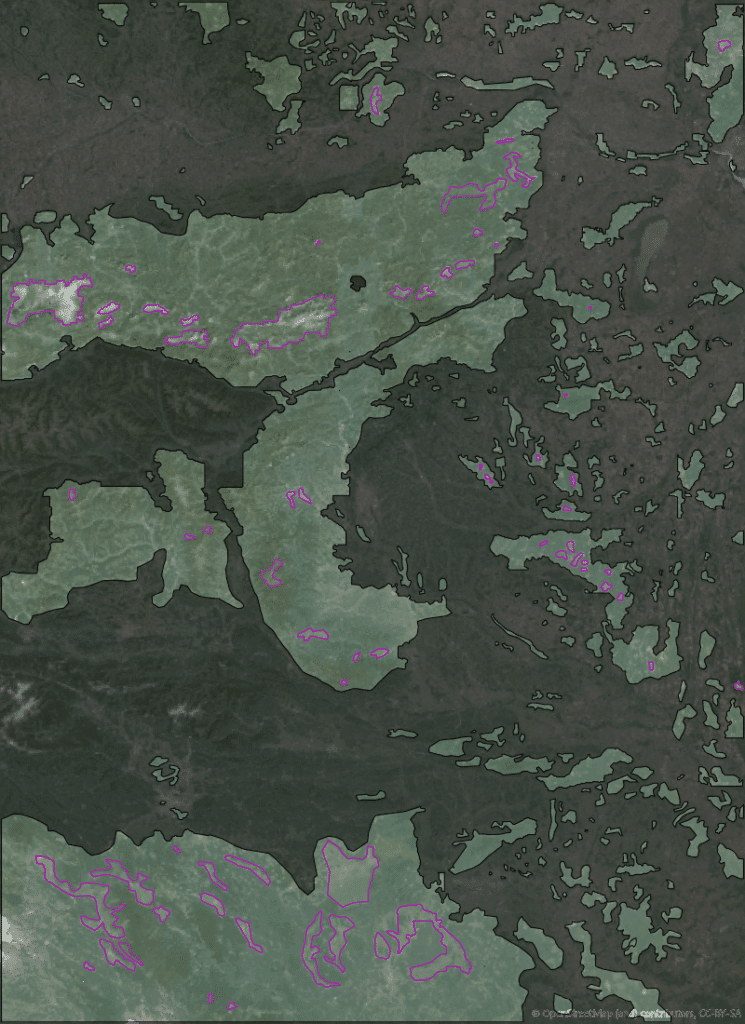
Each site is analysed using 30×30 km tiles (90,000 ha) of Copernicus VHR mosaics (approximately 2 m), which are delivered via WMS and processed to meters for consistent area and edge reporting.
INSIGHTS ON AUSTRIA
The same metrics read like very different landscapes across all six tiles. In Ybbs, Unit 1 is largely intact, consisting of a forest-dominated area with only a few large cuts (mean area ≈ 113 ha, largest area ≈ 1,399 ha, mean shape index ≈ 1.3). Although integrity remains high (LCC ≈ 81%), edges are encroaching on the interior, causing the core area to shrink from 71% to 65% within a 200 m buffer (Δ 6%). The weak spots are the narrow connectors along the main block — any new harvesting should be contiguous and well away from these pinch points. Unit 2 has lighter logging overall, but a less favourable configuration: integrity decreases (LCC ≈ 57%), and the forest is highly sensitive to edges (core area shrinks from 58% to 40% within a 200 m buffer, a decrease of 18 percentage points). Two critical bridges (NSCP = 2) carry much of the connectivity, so the priority is to widen these links and avoid creating new roads across the necks.
In Bad Sankt Leonhard, Unit 1 has a few large, irregular openings (mean area ≈ 99 ha, largest area ≈ 620 ha, MSI ≈ 1.45). The largest connected component remains strong (approximately 82%), with moderate edge sensitivity (core 66% → 54%, Δ 12 percentage points). Unit 2 is even more coherent (LCC ≈ 88%), with a very low clearing share (approximately 0.5%) and only modest core loss (72% → 62%, Δ 10 pp). Here, the main task is to protect the single existing bridge.
Around Graz, Unit 1 features a few large linear openings (mean area ≈ 117 ha, largest area ≈ 520 ha, MSI ≈ 1.30), while maintaining decent integrity (LCC ≈ 78%). Preserving the structure will require keeping the three corridors open (NSCP = 3) and avoiding pinch points. Unit 2 is more fragmented, with a smaller main block (LCC ≈ 63%) and higher edge sensitivity (core 61% → 45% at 200 m, Δ 16 pp), despite relatively little area being cleared. This means that investments in connectivity would deliver outsized benefits here.
In summary, the volume of timber removed has little impact on forest cover at the tile scale, but where those cuts are placed has a significant effect on integrity.
USE-CASE
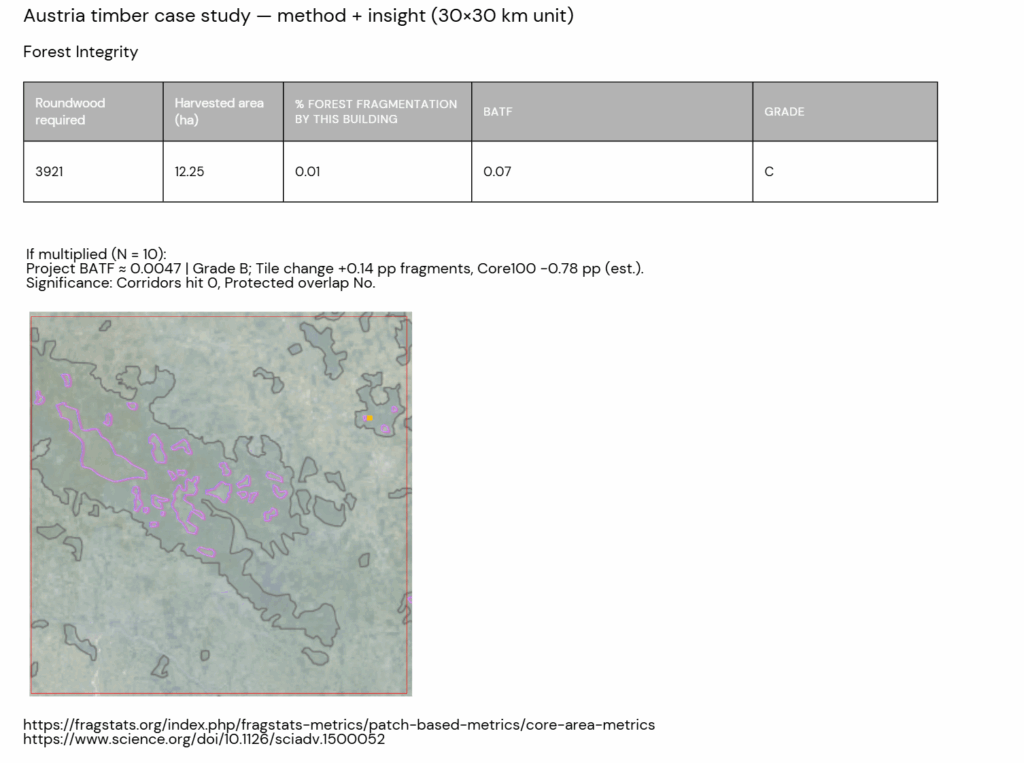
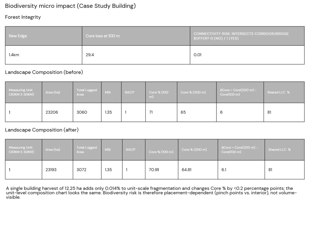
To illustrate the scale, we tested a single Tamedia building: 2,000 m³ of finished timber. Converted to roundwood with a mill yield of 0.60 and a log yield of 0.85, and assuming a harvest intensity of 320 m³/ha, this equates to approximately 12.25 hectares of equivalent harvest. The location of the harvest is far more important than the volume: if you cut it as one block inside the forest interior, you create about 1.4 km of new edge and ~29 ha of 100 m core loss. However, if you split the same volume into ten smaller removals tucked along existing edges, the per-building impact falls to ~1 km of new edge and ~18 ha of core loss. Same wood, very different ecological outcome.
DISCUSSION
We incorporate these trade-offs directly into the design workflow. Inside Grasshopper, the canvas streams live metrics — little pies, bars and counters — while you move a footprint or adjust a sourcing radius. We keep the mean FAD at or above 0.40 across the sourcing window by default to preserve continuous forest conditions, and we apply a no-net-loss rule to the core. We only advance options where the 100–200 m core share is maintained or improved (and we add 10–20 m regreening strips where edges creep in). We protect corridors by maintaining or widening the narrowest links (20–50 m), and we try to minimise NSCP so that the landscape isn’t dependent on a few fragile bridges. Whenever possible, we favour contiguous, compact removals over many scattered micro-cuts to keep edge density in check. These are planning heuristics, not hard limits — local species and habitats always have the final say.
Under the hood, the current model runs on a small, curated set of around 200 samples. To avoid leakage and bias, we use spatially safe splits, deduplicate low-entropy look-alikes and manually label ‘hard cases’. This process increased the F1 score by around 15 percentage points, although small or low-contrast clearings remain the most challenging aspect to get right — a common issue in segmentation. Operating thresholds are derived from precision–recall and F1-confidence curves, and we freeze versions for scenarios to ensure that comparisons remain consistent.
WHY IT MATTERS?
Timber Trace redefines ‘sustainable timber’ as a spatial issue, not just a carbon one. By analysing the structure of forests — edges, cores, perforations and connections — it incorporates biodiversity risk and landscape integrity into the same place where designers already make choices: the early-stage model. This makes it possible to ask and answer the important questions: if this much housing requires this much cross-laminated timber (CLT), what logging would that imply? What would be the associated biodiversity risk? And how would the situation change if we sourced materials differently or repaired key corridors?
Credits. Timber Trace is a Master of Advanced Computation and Design thesis (2025) at IAAC by Giorgia Wolman and Lennart Hamm, supervised by Gabriella Rossi. The methods, study sites, metrics and case study are documented in the thesis booklet and presentation.
