INFOTO

Objective | Information from a Photo

Photos are widely used to quickly capture context but are not easy to relate to spatial data. To remedy this challenge for users of 3D modeling software, we created a tool that integrates Python and Grasshopper to extract the location and time information from a photo and output variable buffers, isochrones, and site features as GeoJSONs and feature summaries as CSVs. This tool vastly expedites the data collection and site analysis and improves coordination among urban development teams.

Methodology | How does it work?

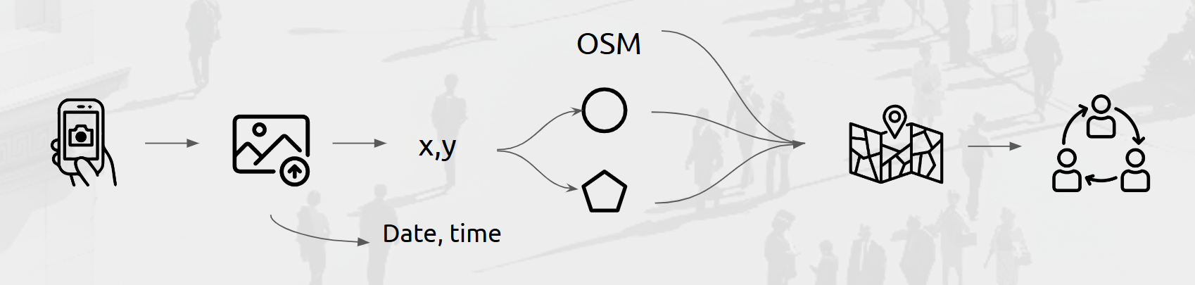
Photos, in this case JPGs, JPEGs, or PNGs, contain EXIF data. This data can be extracted for the photo’s location information and the date and time the photo was taken. This information allows photos to automatically be placed within their context. The coordinates serve as the origin for buffers of a set distance, preset at 500m, or isochrones measuring distance it takes to walk at a set time and speed. To contextualize the user’s site, OpenStreetMap features can be pulled within the resulting buffer or isochrone geometries. For ease of use, we created three options for feature selection: basemap, standard, and detailed. These options are composed of dictionaries of OpenStreetMap keys. The layers of information are exported as GeoJSON files to a set folder path and coallated summaries of features are exported to csv summarized by OpenStreetMap key and value.

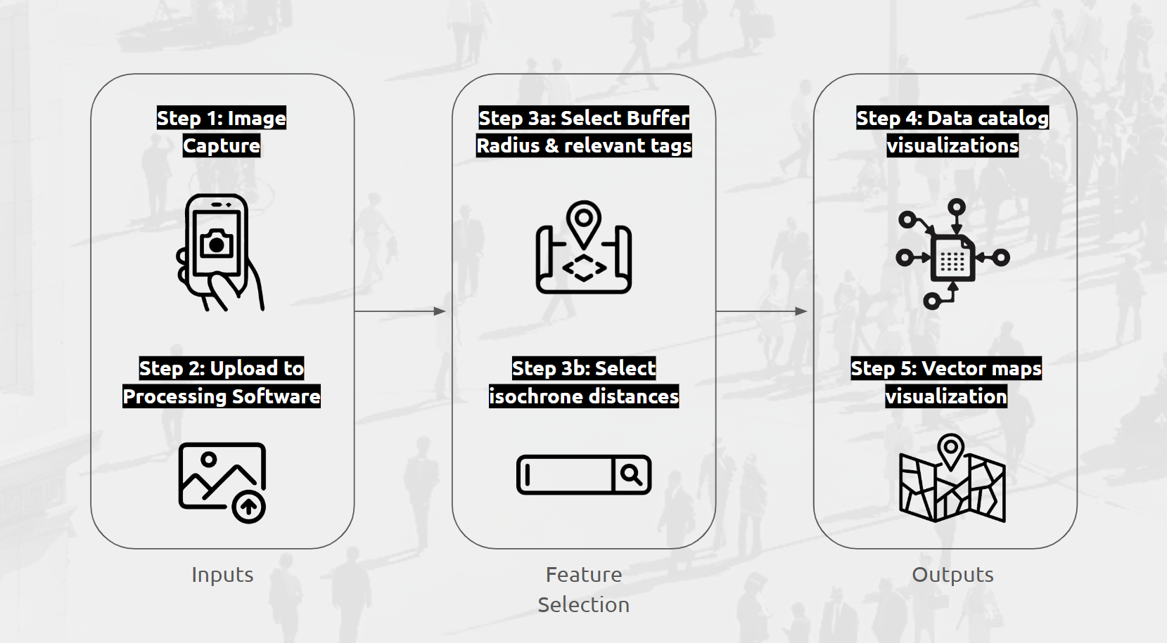
• Step 1-2: EXIF Data Extraction:
  • Goal: Extract GPS metadata from an image.
  • Method:
    • Open the image file using the Python Imaging Library PIL.
    • Verify and extract EXIF data.
    • Extract GPS information from the EXIF data, converting GPS coordinates to degrees for latitude and longitude.
• Step 3a: Buffer Creation:
  • Goal: Create a buffer around a given GPS point.
  • Method:
    • Convert buffer radius from meters to degrees.
    • Create a buffer polygon using the Shapely library.
    • Output the resulting geometry to a GeoJSON file to be saved at the output path.
• Step 3b: Isochrone Generation
  • Goal: Create an isochrone (area reachable within a specified walking time and speed) around a given GPS point.
  • Method:
    • Define a function to calculate the walk isochrone based on the walking time (km/h) and speed (meters/min).
    • Create a graph from OSM data for walking.
    • Find the nearest node to the point location in the walking graph.
    • Calculate the isochrone by determining the subgraph of walkable areas within the specified distance using the NetworkX library.
    • Generate a convex hull polygon reperesentative of an isochrone and store it as a GeoDataFrame.
    • Output the resulting geometry to a GeoJSON file to be saved at the output path.
• Step 4: OSM Data Retrieval:
  • Goal: Retrieve OSM features within the buffer or isochrone area.
  • Method:
    • Use the OSMnx library to query OSM data within the specified polygon.
    • Dynamically adjust the tags for OSM features based on user selection (e.g., Basemap, Standard, Detailed, Custom).
    • Clean the OSM data to handle any list-type columns appropriately.
• Step 5: Ouputting Data
  • Data Summarization:
    • Goal: Summarize building and amenities data from the retrieved OSM features.
    • Method:
      • For buildings, calculate areas and group by building types to get counts, total areas, average heights, and levels.
      • For amenities, group by amenity type to get counts.
  • Visualization and Export:
    • Goal: Visualize and export the geospatial analysis results.
    • Method:
      • Use GeoPandas to save the buffer and OSM data as GeoJSON files.
      • Use Matplotlib for visualizing the buffer and amenities data.
      • Save summarized data as CSV files in the specified output folder.

This simple feature set can be enhanced to increase the flexibility of the user’s analysis. Data catalogs of OSM features can be tailored to the user’s specific needs by accessing the TagInfo API for listed keys and values.

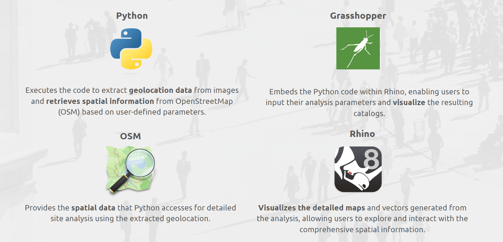
Various tools are used to streamline the process of extracting and visualizing spatial information from site images:

User Interface | How to Run the App

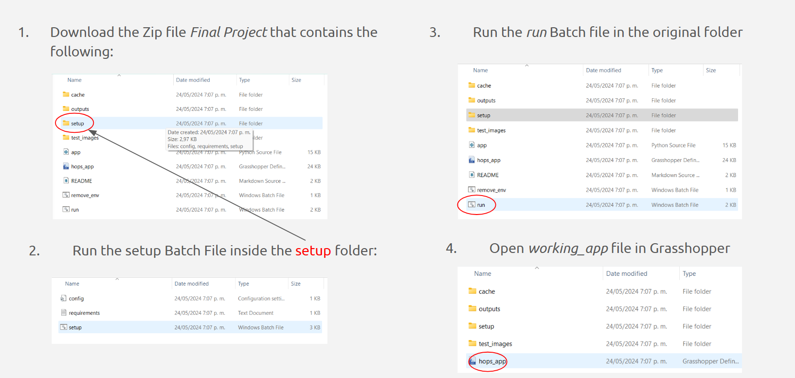
To run the app, first download a zip file of the app contents. Then, find the README which contains instructions on setup, tips on usage, and component logics. Component logics are configuration of components for specific outputs.

Required Plug-ins for grasshopper (available in Package Manager):

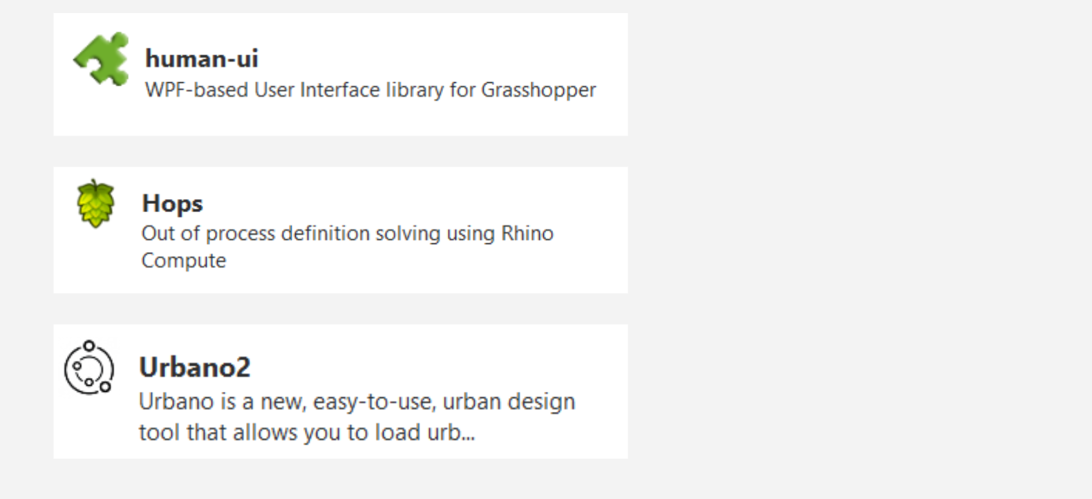
OSM Data Retrieval: BUFFER

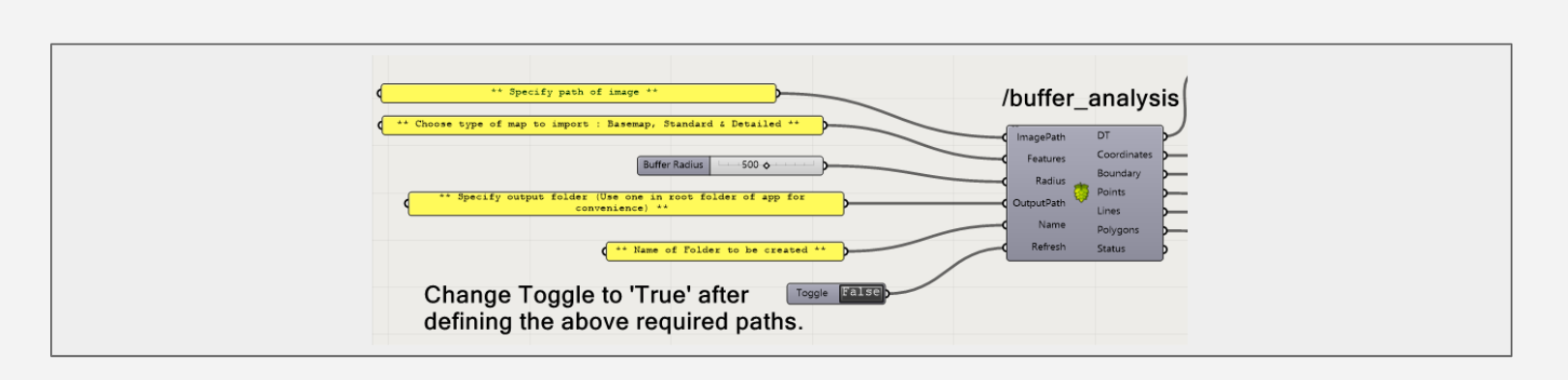
User Interface Components:

• ImagePath: Space for the user to input the path to the image to be used for analysis.  
• Features: Space to select the type of map to import:
  1. Basemap:  Displays essential map features including amenities, buildings, highways, and parks.
  2. Standard: Provides a comprehensive view with buildings, amenities, natural features, land use, and transport networks.
  3. Detailed: Offers an in-depth map with detailed building attributes, amenities, natural features, land use, and extensive transport information.
• Radius: Buffer radius for the spatial data collection.
• Output Path: Space to input the folder path for shapefiles to be stored. 
• Name: Name of the folder to be created.
• Refresh: Turn on button for the collection of data. Only to be turned on when the other information has been provided.

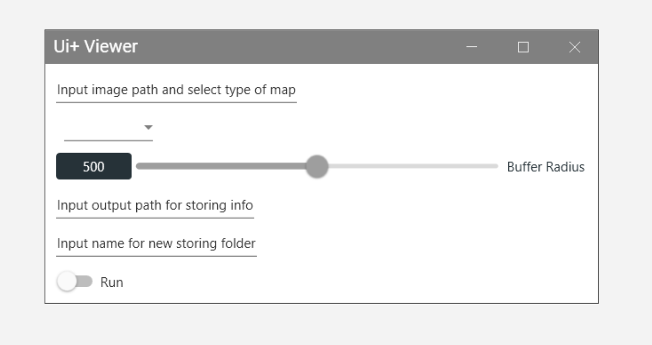
OSM Data Retrieval: ISOCHRONE

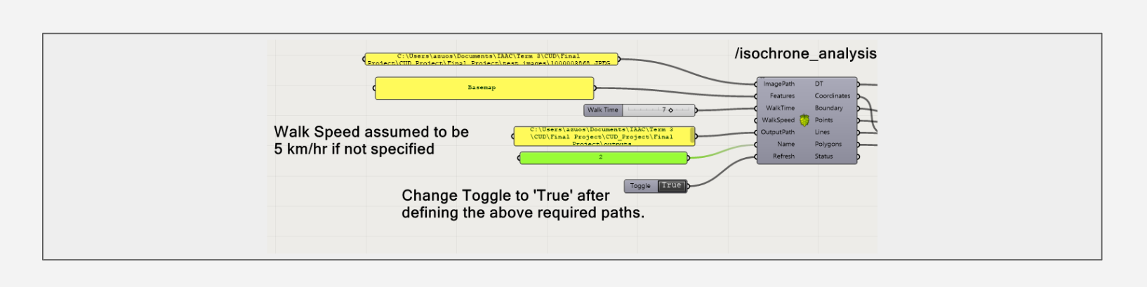
User Interface Components:

• ImagePath: Space for the user to input the path to the image to be used for analysis.  
• Features: Space to select the type of map to import:
  1. Basemap:  Displays essential map features including amenities, buildings, highways, and parks.
  2. Standard: Provides a comprehensive view with buildings, amenities, natural features, land use, and transport networks.
  3. Detailed: Offers an in-depth map with detailed building attributes, amenities, natural features, land use, and extensive transport information.

• WalkTime: Time in min for the isochrone calculation, the extent of the buffer based on how long it takes for a human to reach their destination.
• WalkSpeed: Walking speed for the isochrone calculation. It’s assumed 5 km/hr when not specified. 
• Output Path: Space to input the folder path for shapefiles to be stored. 
• Name: Name of the folder to be created.
• Refresh: Turn on button for the collection of data. Only to be turned on when the other information has been provided.

Implementation and Visualization

Buffer Analysis

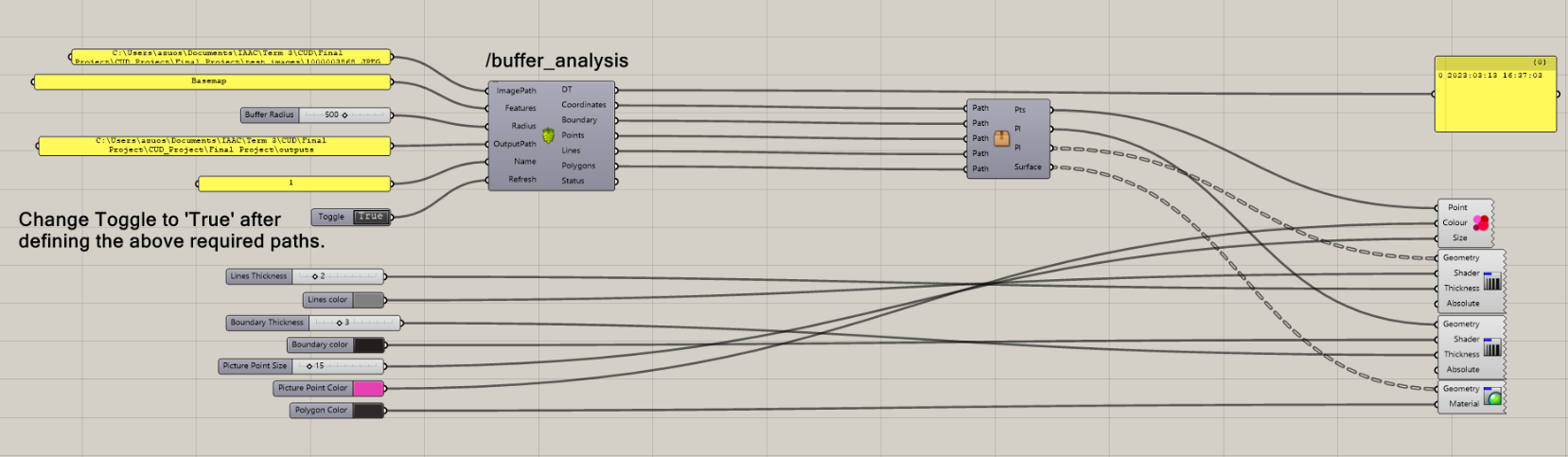
Output

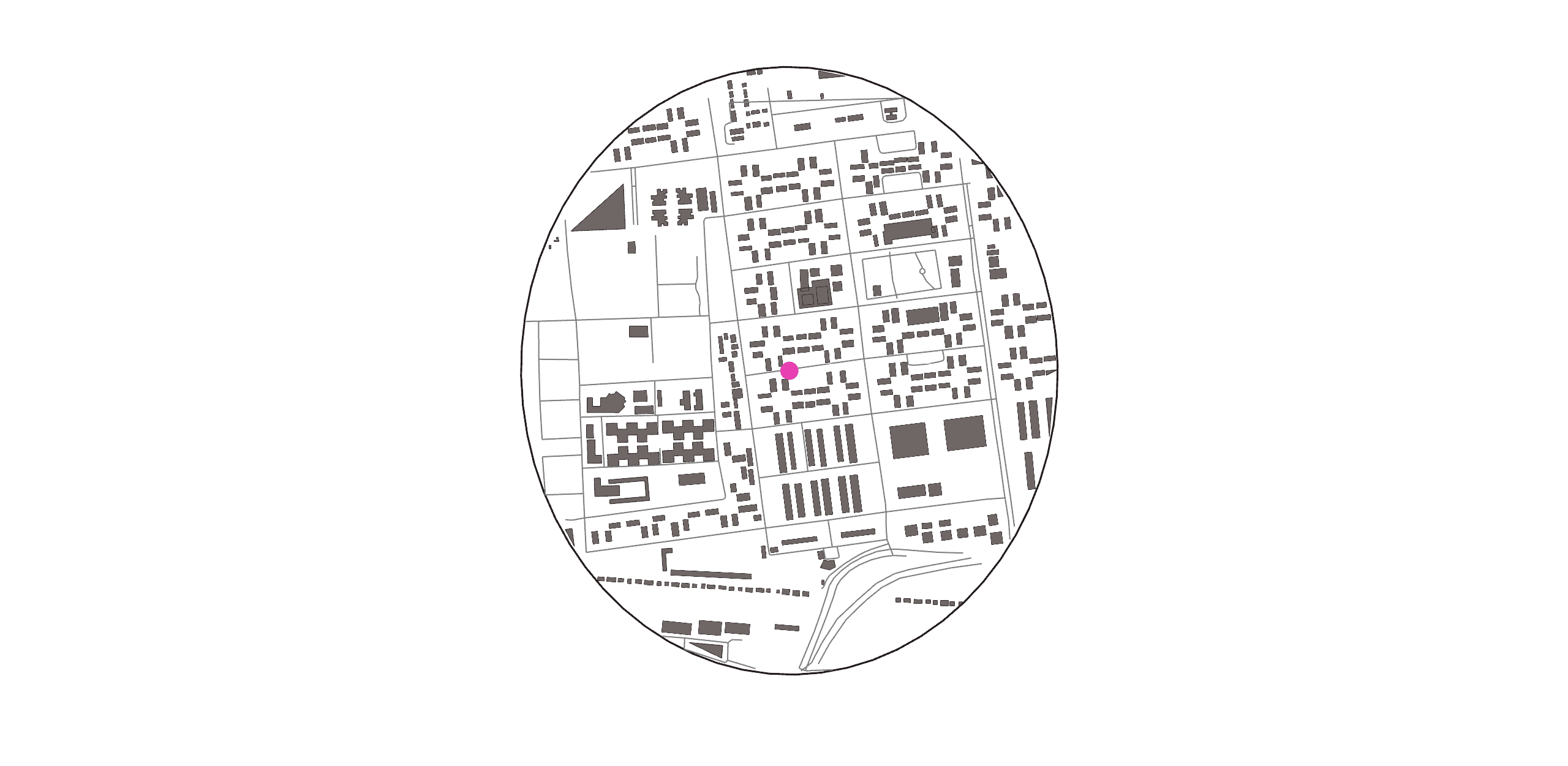
Isochrone Analysis

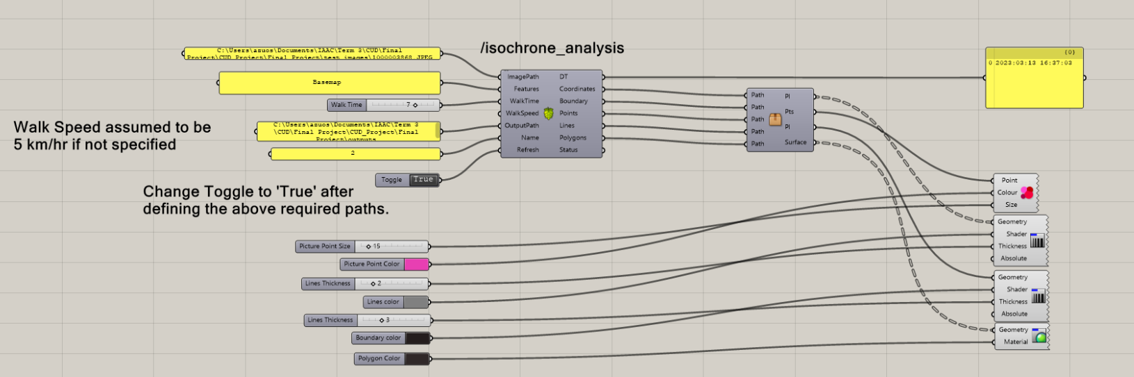
Interface:

Iterations:

Use Cases

1. City Walk: Capture multiple photos while walking through a city to analyze and visualize the surrounding amenities, buildings, and infrastructure along the route.
2. Site Visit: Utilize photos from various points within a large site to assess and map the spatial context and key features, aiding in comprehensive site understanding.
3. Site Selection: Compare features and walkability of different sites by analyzing photos taken from each location to identify differences and similarities in amenities and infrastructure.
4. Urban Development Planning: Collect data from different urban areas to plan and optimize new developments based on existing features and infrastructure.
5. Tourism and Navigation: Use photos from popular tourist destinations to create detailed maps of attractions and routes, enhancing the tourist experience.
6. Safety and Accessibility Audits: Conduct audits by mapping accessibility and safety features in various urban areas to ensure compliance with standards and identify areas for improvement.

Next Steps

This simple module can be enhanced by adding new sources of data and flexibility to the data extraction. The use cases of this tool can be tailored by developing additional dictionaries of OpenStreetMap keys and values.

Sources

• OpenStreetMap
• human-ui
• Hops
• Urbano2
• UI+
• TagInfo