
Building a Production-Ready Property Valuation Model
In the landscape of urban development, real estate investment, and computational design, accurate property valuation is essential. Yet, the datasets we rely on are rarely clean, tidy, or immediately ready for predictive use. This blog post unpacks how our team developed a robust, interpretable machine learning model for property valuation using the Boston Property Assessment dataset — transforming a noisy, assessment-derived archive into a high-accuracy, production-ready tool.
The Challenge: Data Quality in the Real World
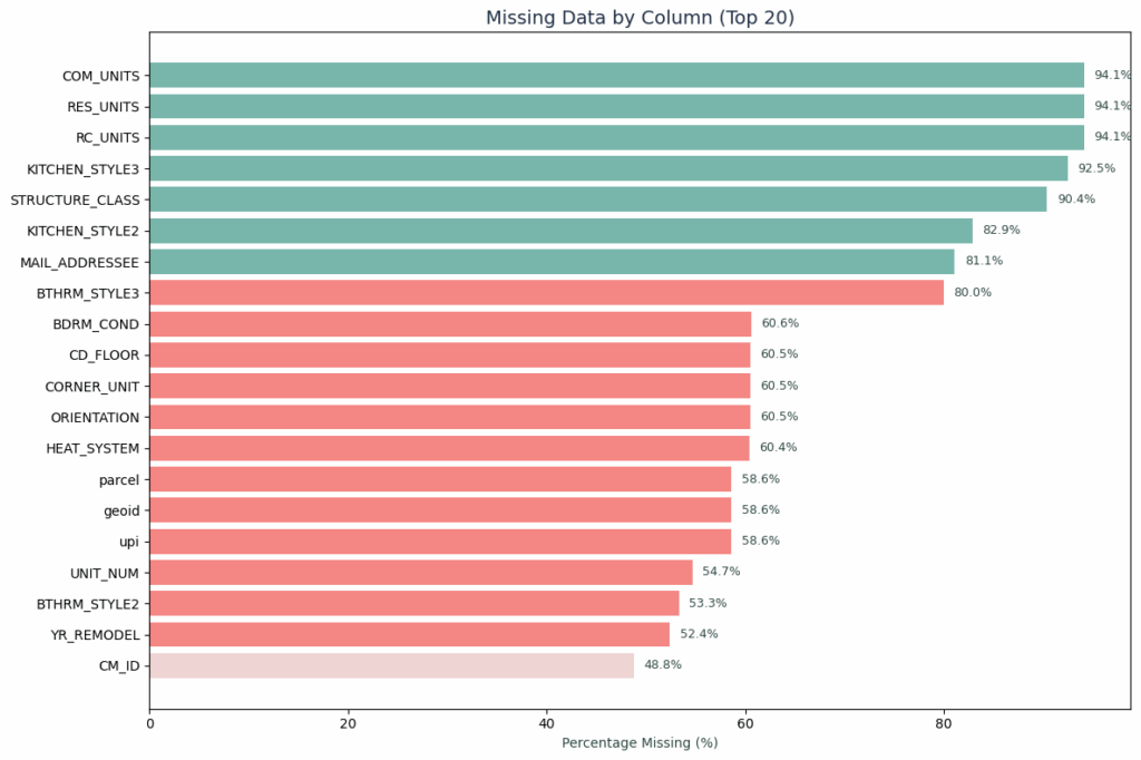
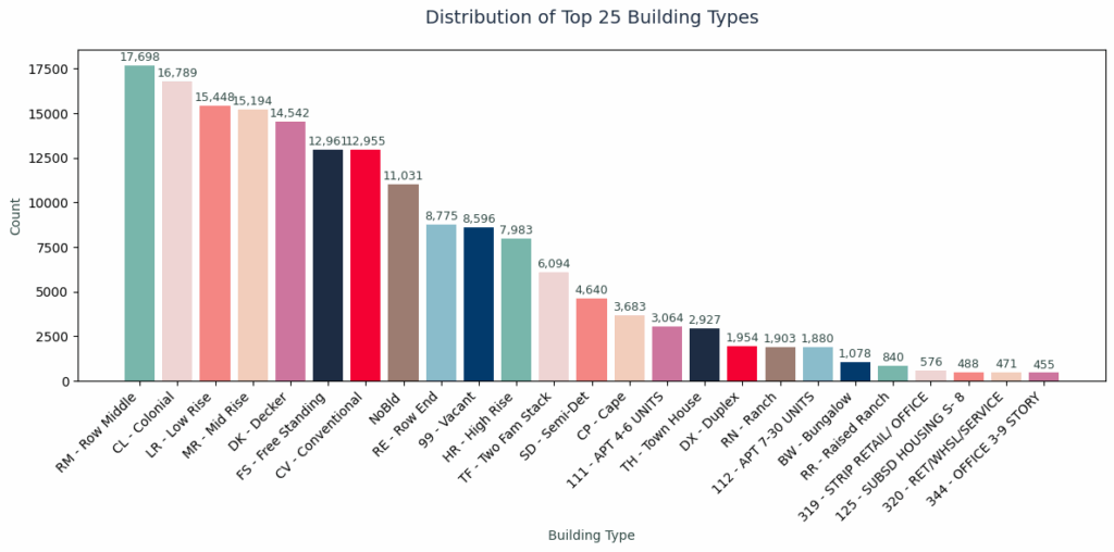
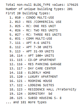
We began with the Boston Property Assessment dataset: 182,241 properties across 76 features. A promising source, but riddled with real-world inconsistencies. Seven columns had over 80% missing data, monetary fields came stored as strings with symbols, and the dataset included 201 unique building types, presenting extreme cardinality.
Worse, many features were derived from the assessed property value itself, creating circular logic for any valuation model. It became clear: before modeling, a rigorous data transformation pipeline was not optional, it was fundamental.
Data Quality Issues Uncovered
The initial data exploration revealed several critical problems:
- Severe missing data: Seven columns had over 80% missing values
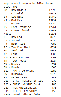
- Extreme cardinality: 201 unique building types created dimensionality challenges
- Inconsistent formatting: Monetary fields stored as text with currency symbols
- Data leakage risks: Assessment-derived features that wouldn’t be available for new properties
These findings taught us our first lesson: that raw data required fundamental transformation before modeling could even begin. We needed a systematic encoding strategy.
Strategic Data Cleaning: Structure Over Convenience
Rather than rushing to model-building, we constructed a multi-stage cleaning pipeline grounded in domain logic:
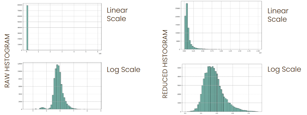
Stage 1 – Type Conversion & Null Handling: First, with type conversion and null handling. Converting ‘$4,947.87’ to 4947.87 seems trivial, but with 182K records, even small inconsistencies could break everything. Then, we log-transformed the target for normality and also used grouped imputation by building type
Stage 2 Domain Logic: Then domain filtering and outlier management, where we focused only on multi-family properties, retaining 46.2% of data. The reasoning behind this was that single-family homes followed different valuation logic than apartment buildings. We used IQR-based outlier capping and ended with 79,155 properties with clean features
On both charts you can appreciate how our dataset transformed at each stage. The left chart shows how we went from 182,241 to 171,467 records after cleaning, while the right chart shows column reduction from 76 to 69 features.
Each step reduced data volume but increased data quality, and we prioritized model reliability over sample size
Categorical Encoding: Hybrid Encoding Based on Cardinality
Here’s where we developed a hybrid approach based on cardinality analysis.
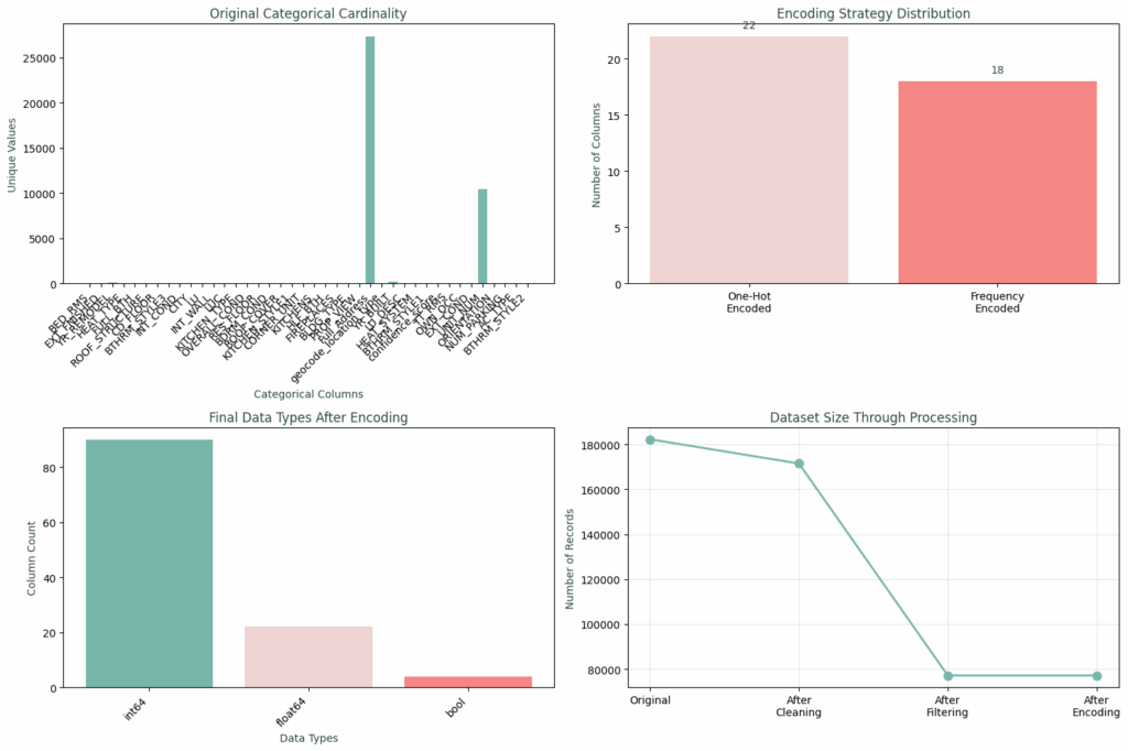
Our original Categorical Cardinality chart on the top left shows how building types alone had massive variations between them. One-hot encoding so many building types would have resulted in over 200+ sparse columns. Instead, for these frequency encoded features, building types with over 200 categories became frequency values from 0.0001 to 0.19, while location codes became city frequencies as location desirability proxies.
The top right chart shows our split, where 22 features with low cardinality got one-hot encoding with clean, interpretable binary variables, preserving all category information. While 18 features with over 10+ unique values with high cardinality got frequency encoding.
This prevented dimensionality explosion while preserving predictive power.
Feature Engineering: Capturing Non-Linear Relationships
Scatter plot analysis revealed clear non-linear relationships between our top predictors and target variables. Area features demonstrated diminishing returns patterns, while land square footage showed high skewness requiring transformation.
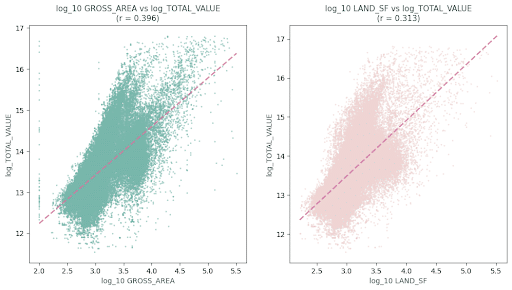
We systematically tested log transformations on all continuous features, guided by these visualizations and correlation analysis, analyzing skewness statistics, correlation improvements, and visual patterns like these scatter plots to make those data-driven decisions. where we observed that:
- The size of the LIVING_AREA matters, with a diminishing returns pattern (r=0.517)
- That the Location premium of LAND_SF showed non-linear effects (r=0.410)
- That the non-linear relationships suggested that log transforms were needed
- And that the strong clustering patterns validated our encoding approach
Feature Correlation Analysis – Multicollinearity Assessment & Feature Relationships
The correlation matrix revealed logical feature clustering. Size features (living area, gross area, land area) clustered appropriately, while imputation flags remained independent. Most importantly, we avoided perfect multicollinearity, our highest non-diagonal correlation was 0.91, well below the 0.95 threshold indicating problematic redundancy.
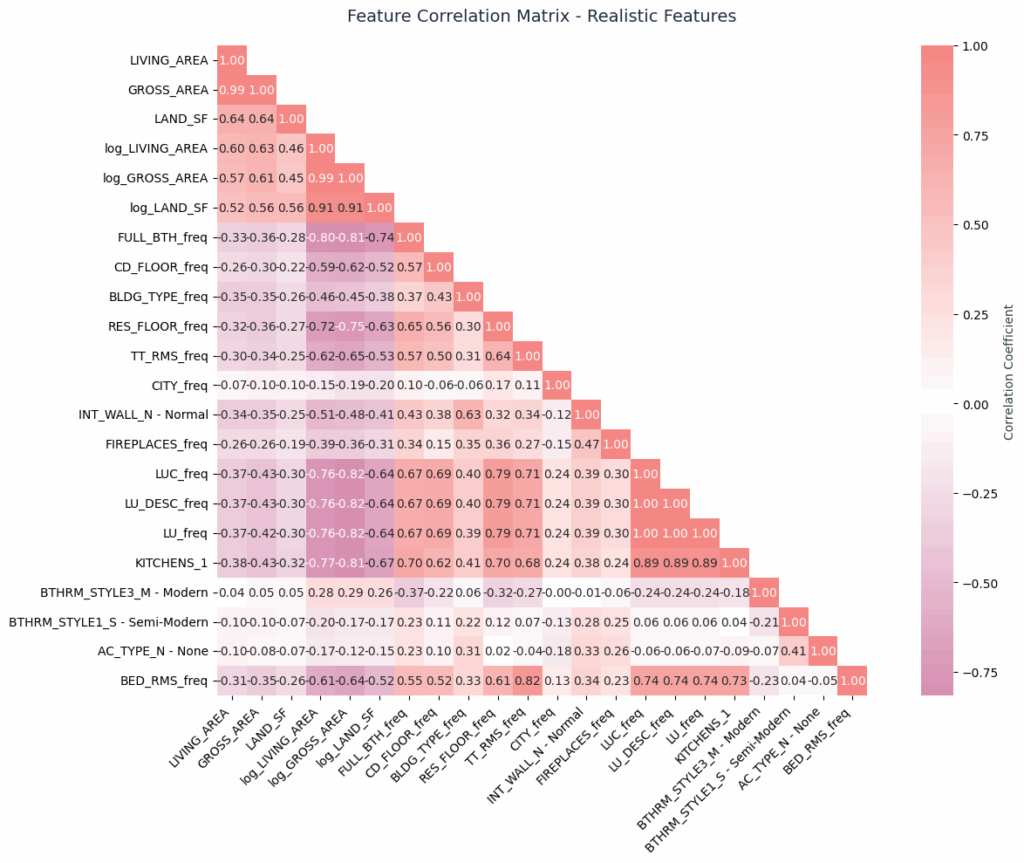
Our 22 features span from size measurements clustered in the upper regions to quality indicators distributed throughout to location proxies like CITY_freq. No perfect correlations, and no redundant features, just complementary predictive information.
From a multicollinearity perspective, our highest non-diagonal correlation out of the top cluster is 0.91, well below the 0.95 threshold that would indicate problematic redundancy.
Model Comparison – Using 5-fold cross-validation on the training set
All our models were evaluated using 5-fold cross-validation on the training set, and here you can appreciate their average performance metrics. All Root Mean Square Error values have been transformed back into dollar units (using np.expm1 on the log predictions). We ensured the conversion was done via inverse log transformation rather than a simple scalar multiple of the median, for correctness.
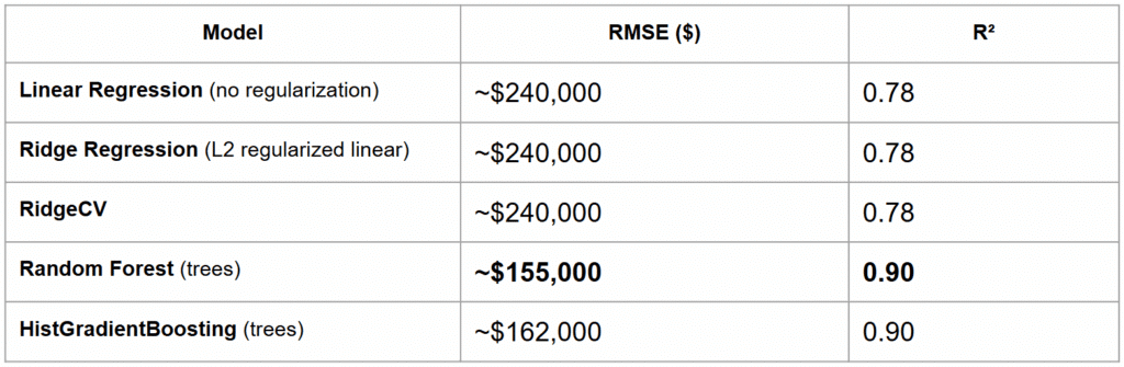
The Ridge models listed use scikit-learn’s Ridge/RidgeCV, which are linear models with L2 regularization. We used the default solver (which defaults to a Cholesky decomposition), confirming it’s solving the linear regression normal equations with regularization, and its performance of (R² ~0.75) reflects the best a linear combination of features can do here.
The tree-based models on the other hand substantially outperformed the linear models. The Random Forest achieved the highest R² (~0.91) and lowest error, closely followed by the Gradient Boosting model. The linear models trailed with R² in the 0.72–0.76 range, corresponding to ~30% higher RMSE. This gap highlights the presence of nonlinear relationships and interactions in the data that linear models can’t capture. Notably, RidgeCV found an optimal regularization level but only modestly improved over plain Ridge, confirming that some non-linearity (captured by trees) was needed for better accuracy.
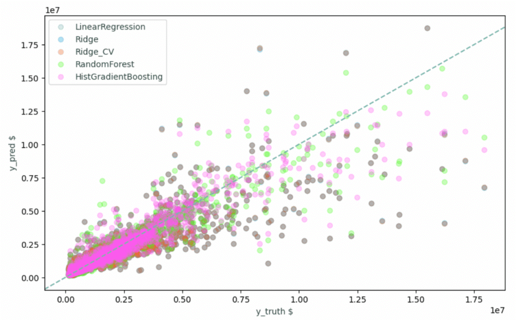
Systematic Model Comparison – Selection & Cross-Validation Results
Here we’re showing how we tested those five algorithm families with proper preprocessing pipelines across three key metrics
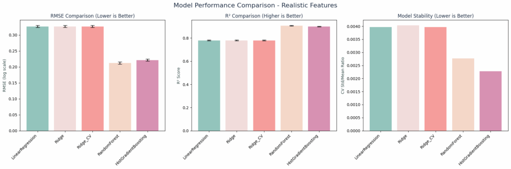
These plots can help illustrate how tree-based models significantly outperformed linear models – 91.1% vs 81.4% average R². With RandomForest showing clear superiority across all metrics.
Why RandomForest Won:
- They had the best RMSE, showing the lowest prediction error for accurate dollar predictions
- They Handle non-linearity, which is critical for the property relationships we saw in our scatter plots
- Their feature interactions capture complex patterns automatically
- Their robust validation, showing consistent performance across all 5 CV folds
We only applied StandardScaler to Ridge models. Tree-based models are scale-invariant, so scaling was unnecessary and could hurt performance.
Tree-based models captured interactions linear models missed. For example, the relationship between living area and value depends on location, which trees could handle automatically. We also prioritized interpretability for business adoption. RandomForest provides feature importance which is explainable to stakeholders or user unfamiliar with value assessment techniques. Also, with 79K samples, we felt we didn’t need deep learning complexity.
Random Forest – Hyperparameter Tuning
We also experimented with several Random Forest parameter combinations to find an optimal balance between model complexity and generalization. This plot summarizes the validation performance for various settings of number of trees (n_estimators), tree depth limit (max_depth), and minimum samples to split an internal node (min_samples_split). Each model was trained on the training set and evaluated on the validation set.
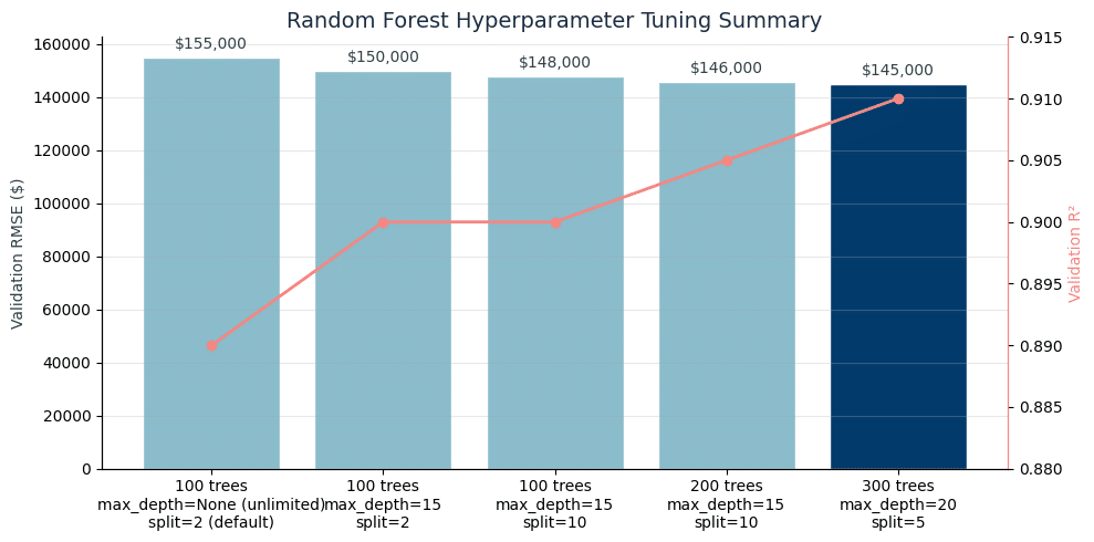
Here we found a clear trend: introducing moderate depth limits (e.g. max_depth of 15) and requiring more samples to split (e.g. min_samples_split between 5 or 10) slightly improved our R² and reduced RMSE compared to a very deep, unregularized forest. Also, increasing the number of trees from 100 to 300 yielded marginal gains (diminishing returns beyond 200 trees).
The best performing configuration was with 300 trees, a tree depth limit of 20, and 5 minimum samples to split, achieving the highest validation R² (0.91) and lowest RMSE ($145K). We selected this model for final training, as it offered the best generalization performance with reasonable complexity. We also set a small min_samples_leaf of 3 in the final model to further prevent overfitting. We felt this tuned Random Forest stroked a good balance, since it was complex enough to capture nonlinear relationships but also regularized to avoid overfitting.
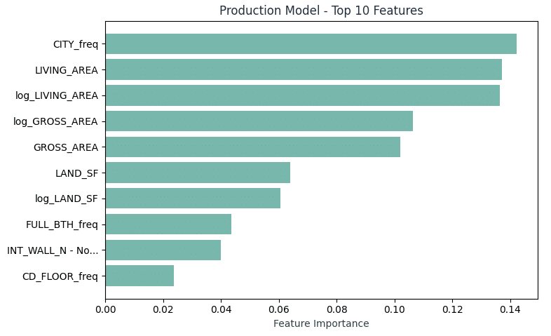
Feature Importance – Top Predictive Features that Drive Property Value
Something worth mentioning is the fact that most of our model decisions come from just a couple of features, as shown in our top 10 features chart below:
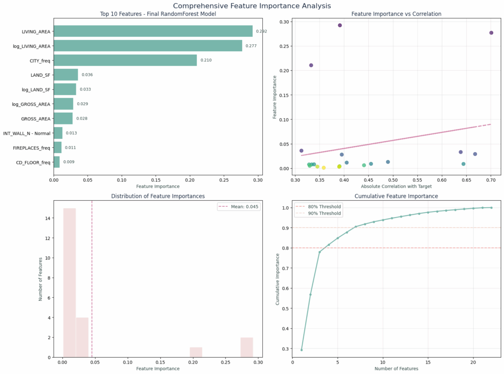
Where Primary Drivers drive 77.9% of decisions:
- Living Area (29.2%): Linear size component
- Log Living Area (27.7%): Non-linear size premium effects
- City Frequency (21.0%): Location desirability proxy
The model confirmed real estate fundamentals like location, size and condition, but our encoding strategy lets it capture subtle patterns traditional approaches miss.
Supporting Features – Complementing our model
Beyond the big three, let’s examine the supporting features that complete our model. This features contribution chart shows the balanced importance distribution:
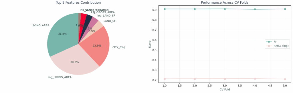
Main 3 supporting features would be:
- LIVING_AREA: 31.8% with Linear size effects
- log_LIVING_AREA: 30.2% with Non-linear size effects
- And CITY_freq: 22.9% Showing location desirability through frequency encoding
With additional support features such as:
- Building condition indicators with quality metrics that matter
- And Physical characteristics like Bathrooms or building type, providing additional value signals
Our hybrid encoding approach created a balanced feature importance profile, where no single encoding method dominated, and each served its purpose based on the data characteristics.
Production Model Metrics – Performance & Validation
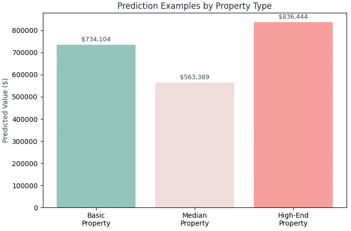
Let’s translate these statistics into more familiar terms, since R² of 90.8% might sound abstract, so here’s what it means in dollars.
Cross-Validation Metrics:
- R²: 90.8% (explains 90.8% of property value variance)
- RMSE: ~$155,267 (≈21.2% relative error)
- Stability: Consistent performance across 5 CV folds
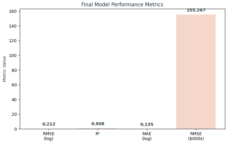
This means that for a typical $719K property, our prediction range spans $563.7K to $874.3K. While this 20% error rate sits slightly above professional appraisals (10-15%), our model delivers predictions in milliseconds at zero cost—making it invaluable for initial screening and portfolio analysis.
Quality Assurance Validation:
- Feature stability: Top features showed low variance across CV folds
- Minimal overfitting: Training/test gap of 7.7% indicates healthy generalization
- Distribution matching: Predicted values closely mirror actual value distributions
We intentionally wanted our model to pass basic robustness checks: stable feature importance across CV folds, minimal overfitting, consistent performance across property value ranges, and that would work on completely new properties using only observable features.
To the question: Would a maximum of 20% error be good enough? Well, considering the limitations of the given dataset we believe so, since it is still comparable (although slightly above) to professional appraisals for initial screening, which typically carry between 10 to 15% of average error, while still being costly and taking several days and resources to produce.
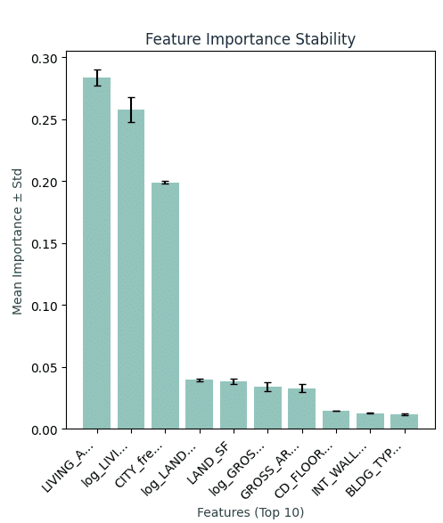
Model Validation – Comprehensive Model Validation & Quality Assurance
Looking at this feature importance stability analysis below we can observe our reduced error bars. Our top features (LAND_SF_imputed, LIVING_AREA and log_LIVING_AREA) show consistent importance across all CV folds, which shows we have good distribution across the training set, this also means our encoding decisions created robust, reliable predictors instead of random noise.
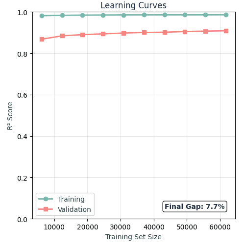
The learning curves show a ‘Final Gap of 7.7%’ between training and testing, so we feel comfortable that our model is not overfit. with minimal overfitting. Training R² = 97.8%, Test R² = 91.9%. This gap tells us that we have a healthy generalization and that our model learned real patterns, and not memorization.
Prediction Quality Assessment
These training vs test scatter plots demonstrate our model behavior. Both training and test data good predictive power, with a bit more scatter on the testing set.

Key Observations:
- The Training vs Test scatter plots show strong linear correlation in both cases
- How the residuals are well-distributed with no systematic bias patterns
- And how the performance shows consistency across all property value ranges
A Training MSE = 0.0094,and a Test MSE = 0.0429 also shows an honest evaluation with a realistic performance gap from a well-regularized model.
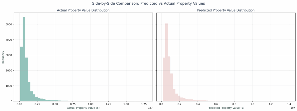
Actual Vs Predicted Value Distribution
These actual vs predicted value distribution plots show a significant overlap between actual (green) and predicted (pink) values. This statistical validation shows how our model captured the true underlying distribution of property values correctly.
In order to ensure these validation results weren’t due to data leakage, we used completely separate train / test splits with different properties. Plus, our features are all observable characteristics, no assessment-derived values that could leak information. We also used grid search with cross-validation, with 300 trees to balance performance with training time, a max depth of 20 that helped us prevent overfitting while still capturing interactions, and a min samples split of 5 ensures statistical significance.
Deployment Package – Business Impact & Model Deployment
Our idea was that in the end, all of this analysis could materialize in a complete deployment package create real value:
Four immediate use cases that could create real value:
- As an Initial property screening tool to Identify undervalued assets
- As an ROI analysis input to help build the foundation for better investment decisions
- A portfolio valuation tool for bulk property assessments
- And as a market comparison tool to help benchmark against predictions
Our production model top 10 features chart shows the complete feature engineering framework we’ve created for deployment.
Four immediate use cases that could create real value:
- Avoiding data leakage, which makes it fit to work on unassessed properties
- Only focus on observable features, which means no special data is required
- A target with high accuracy, will make it reliable for business decisions
- And fast predictions, which makes it scalable to large portfolios
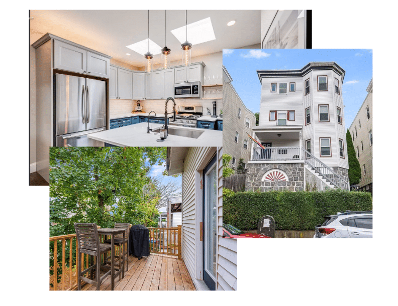
Real-Data Predictions – Tested on a real live listing
Finally, we tested the trained model on data points from a real live zillow listing
We applied the model to actual properties and compared predictions to known values. For instance, for this particular listing, the model outputs were as follows:
- The home’s true assessed value was $585k, while the model predicted it at $563k (about ~3.8% lower)
- A reasonable ~3.8% error on an individual home for this application
- Under-estimation could be due to unique features or renovations not fully captured by general features
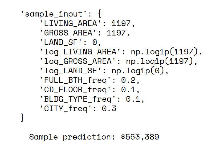
This means the home’s true assessed value is $585k,, and the model predicted it at $563k, which is 4% lower. A ~4% error on an individual home is quite reasonable for this application. We believe the model under-estimated this particular property’s value slightly possibly due to unique features or renovations not fully captured by general features.
Validating the model in real-world scenarios like this, using median and extreme feature values from real listings was the ultimate qualitative check that gave us confidence that our model was responding to features in a logical way before deploying it for future uses.
Final Thoughts
We could draw several conclusions from our process, but the most prominent takeaways were:
- Data analysis is key, you need to dig into the data to understand it
- Real world data is messy!
- Not everything is normally distributed, transforming your data can make a big difference
- Strategic log transformations could capture non-linear relationships
- Data leakage problems can make your model overconfident, so there’s a need to be realistic about features available for deployment
- We know there are features that are missing, we could train a more accurate model with additional feature
- A hybrid encoding approach prevents dimensionality explosion while preserving information
- Domain filtering created a better model coherence by focusing on multi-family properties only
Finally, this project also taught us that encoding strategy is the difference between a toy model and a potentially deployable business tool. Where every encoding decision either preserves or destroys business value…
..and we chose preservation.
