Introduction
Our reference paper is Boeing, G. (2019). Urban spatial order: street network orientation, configuration, and entropy. We Applied Network Science, 4(1), 1–19
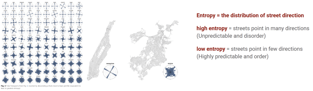
What is Entropy?
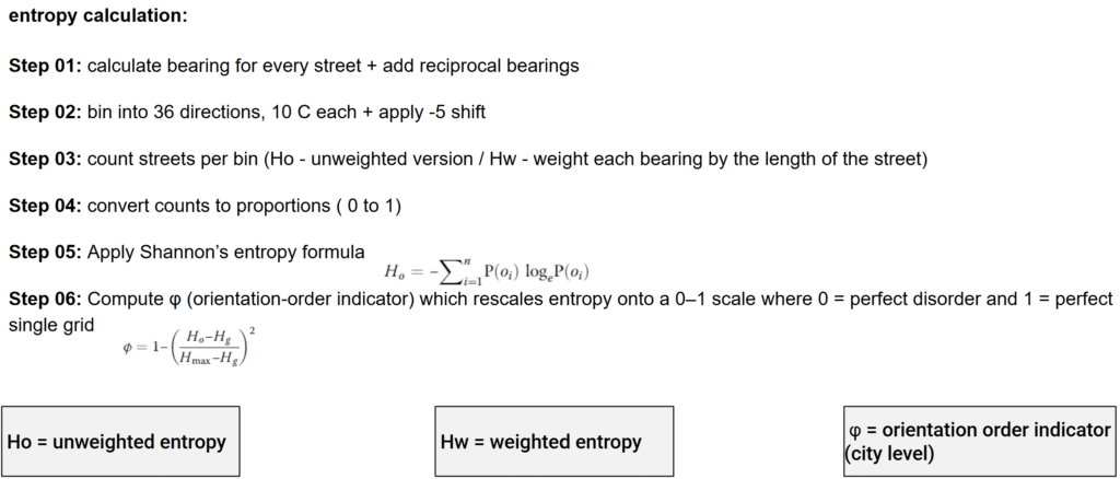
How was Entropy calculted?
After understanding Boeing’s method, our next step was to recreate his workflow and validate our implementation.
One small difference is that we used smaller bin intervals than the original implementation, giving us a slightly finer directional resolution.
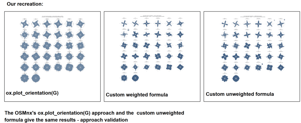
compared our custom unweighted implementation with the Boeing’s OSMnx output, the results were essentially the same. This gave us confidence that our entropy calculation was correctly reproducing the logic from the paper before applying it to our own dataset.
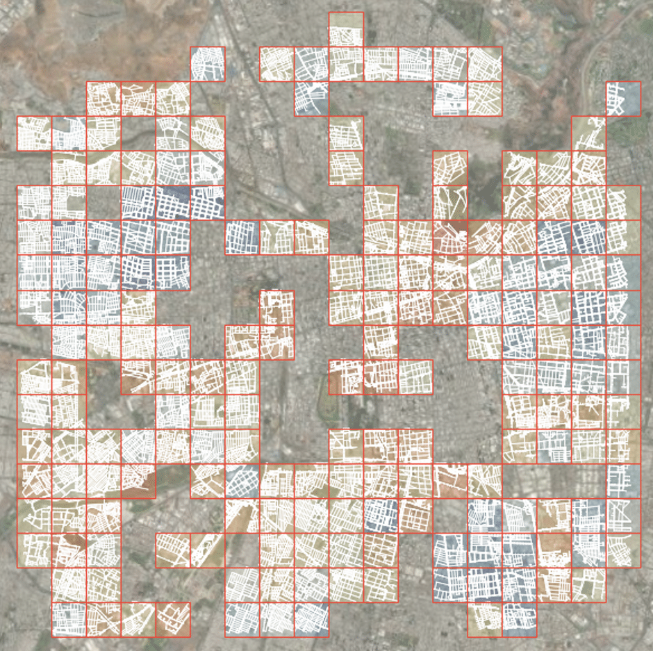
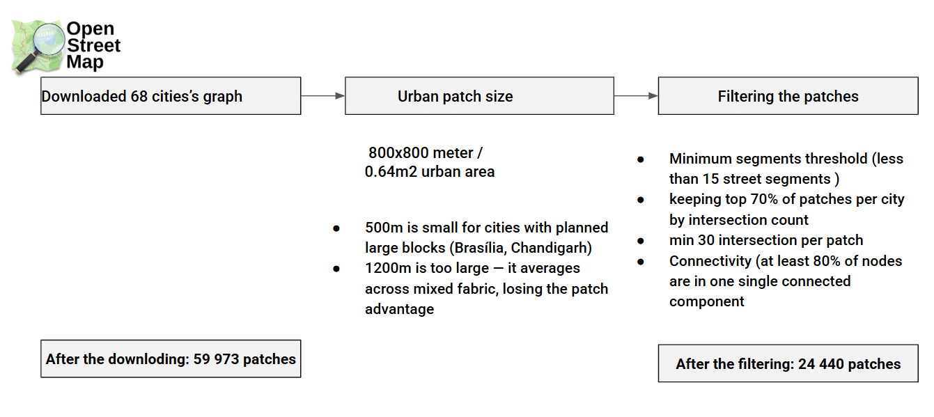
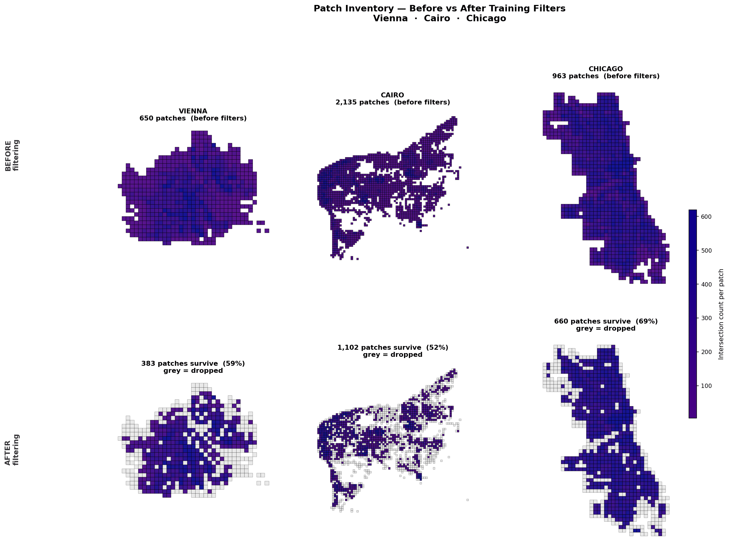
Starting with the raw city
We began by downloading 68 cities from OpenStreetMap and slicing each one into 800×800 m patches, yielding roughly 60,000 patches in total. Most of these don’t represent meaningful urban fabric, so we filtered aggressively, primarily on intersection counts per patch, to discard outskirts, isolated parks, and industrial zones. That left us with 24,440 patches that better capture genuine urban identity. Sampling Vienna, Cairo, and Chicago before and after filtering confirmed the cleanup was doing what we wanted.
Computing entropy and balancing the distribution
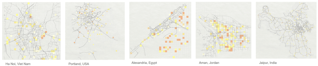
For each surviving patch we calculated street network orientation entropy. A model is only as good as its target distribution, so we aimed for an even spread of entropy values rather than letting the data pile up wherever cities naturally cluster.
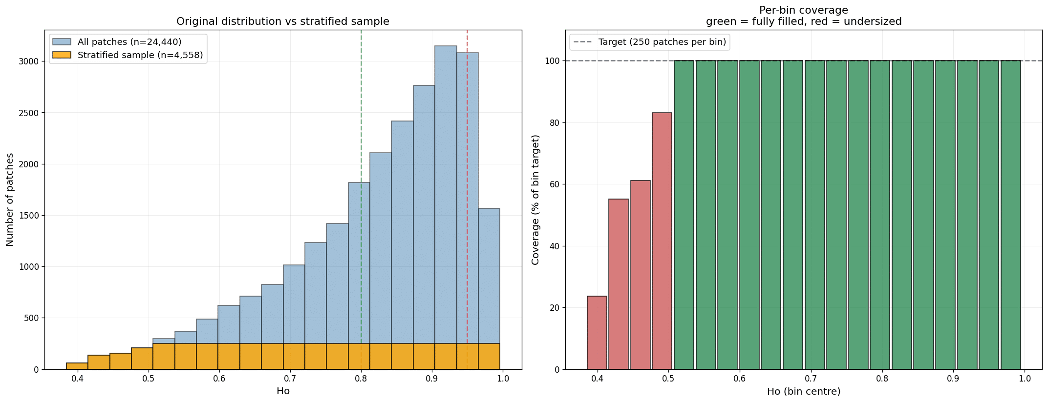
Our first attempt targeted 5,000 patches using 20 bins of 250 patches each. Four bins came up undersized, all of them at the low-entropy end. The fix was to bring in more cities. Three additional cities slightly improved coverage; more cities improved it further. We noticed that North American cities had an outsized effect on the empty low-entropy bins, since their gridded layouts produce low orientation entropy, so we deliberately added more of them.
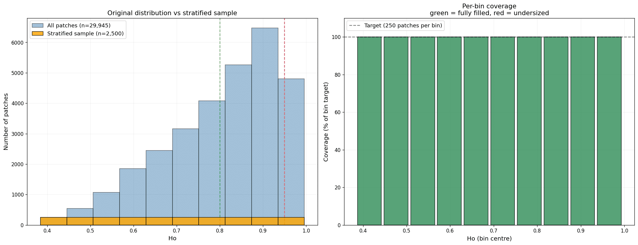
Rather than chase a target the data couldn’t support, we lowered our ambition to 10 bins of 250 patches. The result: a clean dataset of 2,500 patches with an even entropy distribution
Computing graph features
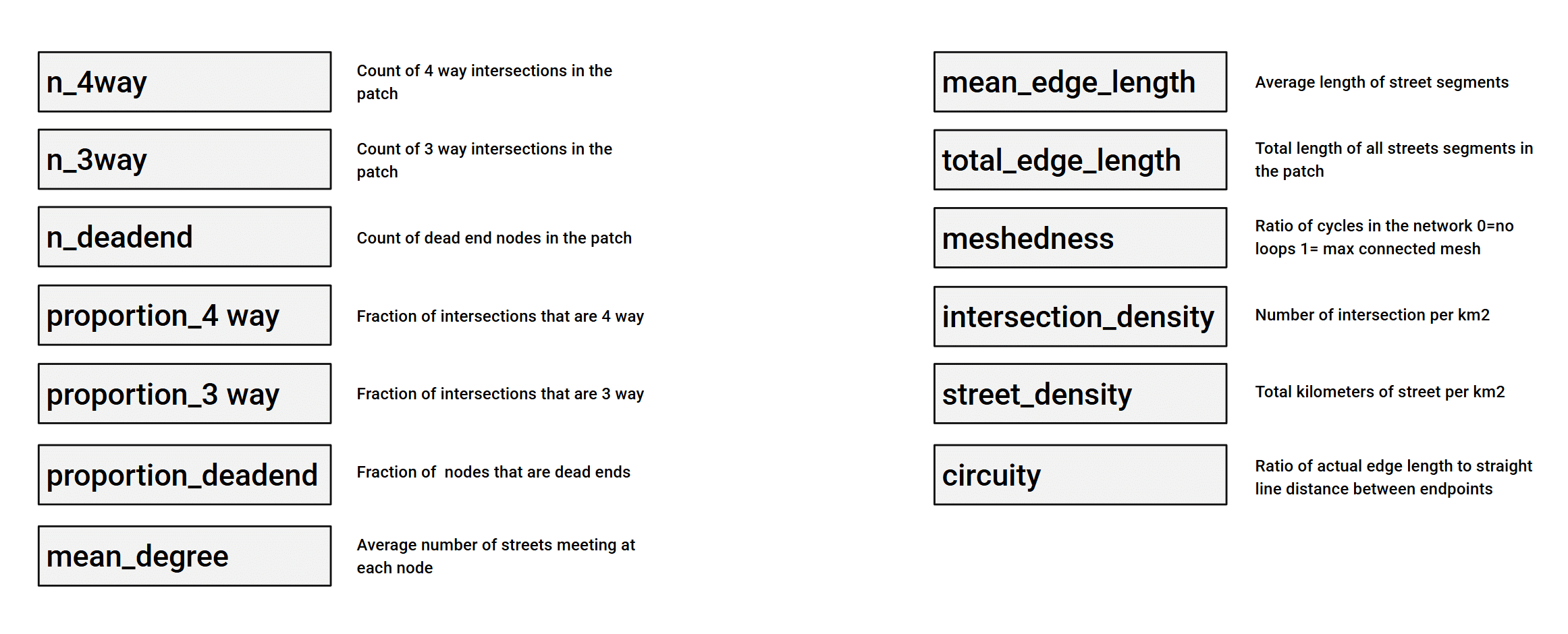
To describe each patch numerically, we computed 13 features from its street network graph, capturing intersection types, connectivity, density, and geometry.
Several features count and characterize intersections. n_4way and n_3way count four-way and three-way intersections, while n_deadend counts dead-end nodes. Their normalized counterparts, proportion_4way, proportion_3way, and proportion_deadend, express these as fractions of all intersections (or nodes), making them comparable across patches of differing size. mean_degree, the average number of streets meeting at each node, summarizes overall intersection complexity in a single value.
A second group describes street geometry and length. mean_edge_length gives the average length of a street segment, and total_edge_length the combined length of all segments in the patch. circuity is the ratio of actual edge length to the straight-line distance between endpoints, indicating how winding or direct the streets are; a value near 1 means streets run straight between intersections.
The remaining features capture connectivity and density. meshedness measures the ratio of cycles in the network, from 0 (no loops) to 1 (a maximally connected mesh), reflecting how many alternative routes the grid offers. intersection_density (intersections per km²) and street_density (kilometers of street per km²) describe how tightly packed the network is.
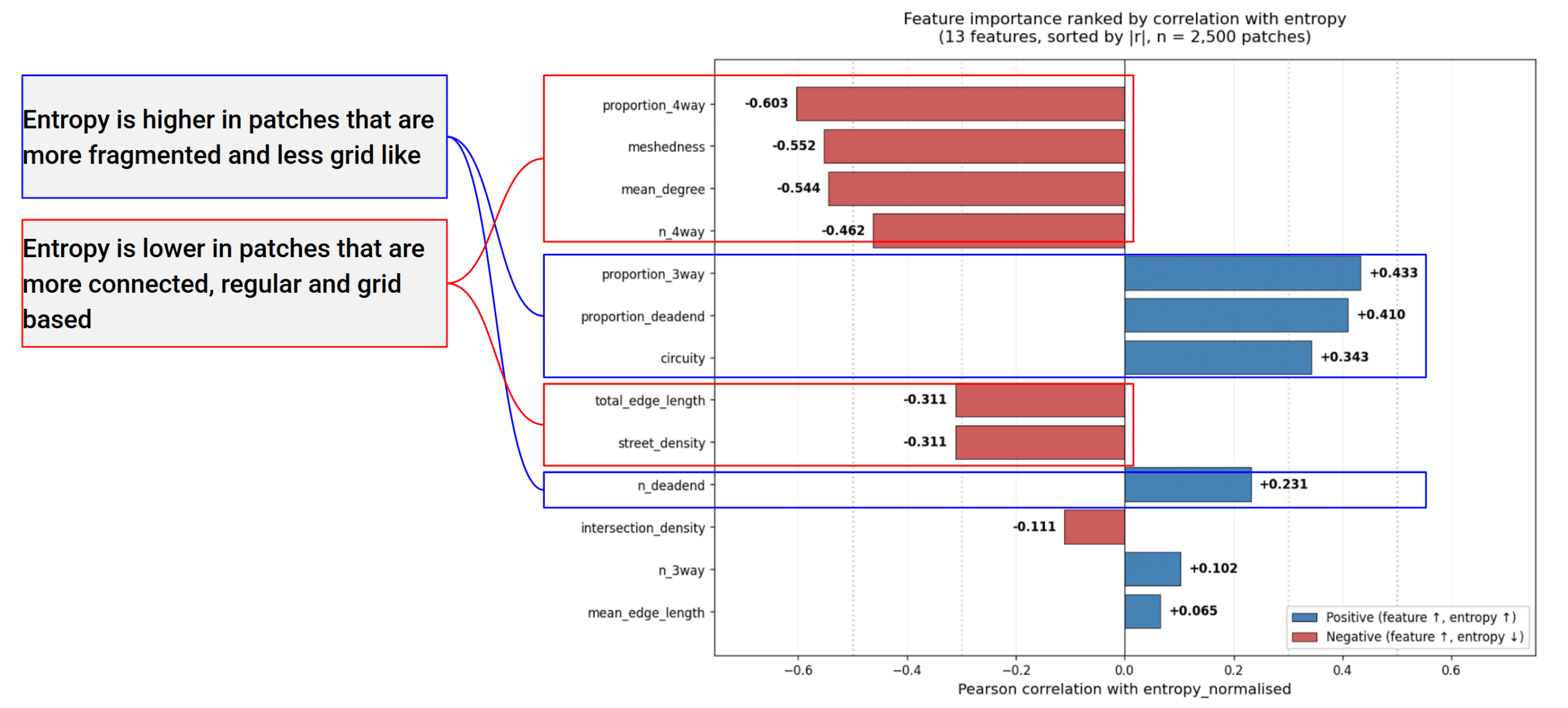
Together these features span the qualities that distinguish urban fabrics: a tight, looping grid scores high on four-way proportion, meshedness, and density with low circuity, while a sprawling, fragmented layout shows more dead ends, higher circuity, and lower connectivity, exactly the kinds of contrasts the entropy target reflects.
Feature engineering
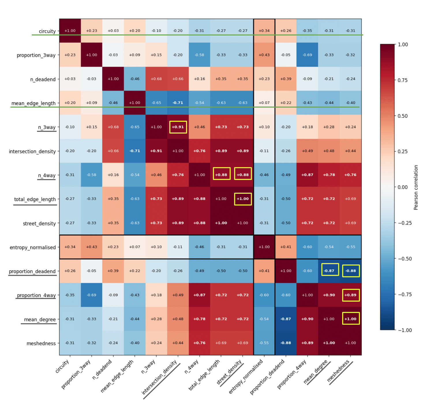
For each patch we computed 13 features describing the urban network derived from the downloaded graphs. Correlating these against entropy was informative: entropy correlated strongly and negatively with features describing fragmentation, and inversely with features capturing connectivity and grid regularity. Lower entropy tracks ordered, connected, grid-like fabric, exactly what you’d expect.
K-means clustering 01
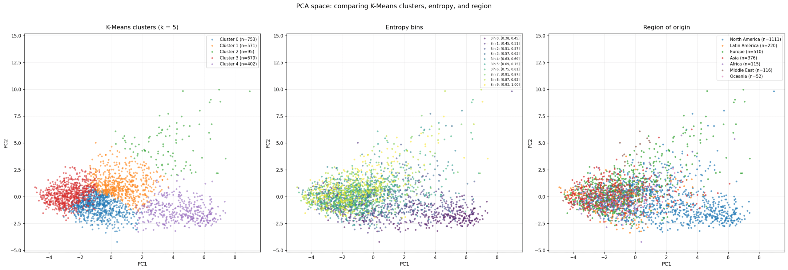
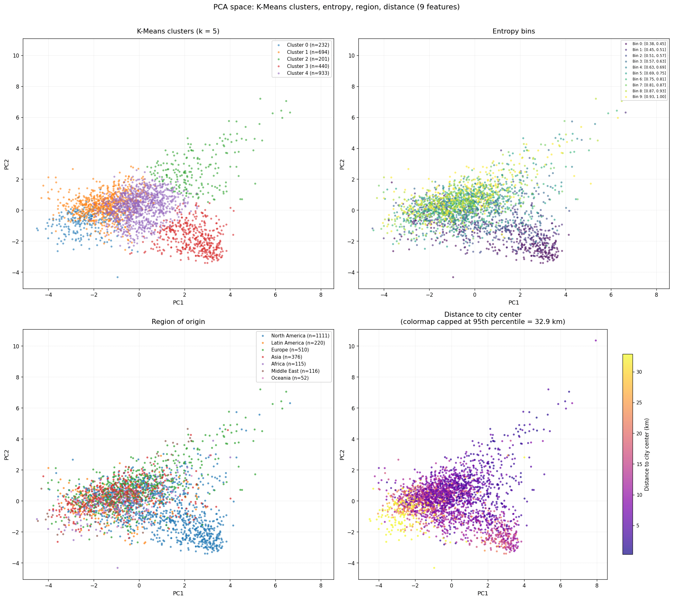
K-Means with 5 clusters showed reasonably clean separation. Coloring by region of origin and by distance to city center (a proxy for city age, since true age isn’t available per patch) revealed two patterns: low entropy follows North American cities, and patches farther from the center clustered loosely enough to suggest distance-to-center was worth adding as a feature.
Feature correlation matrix
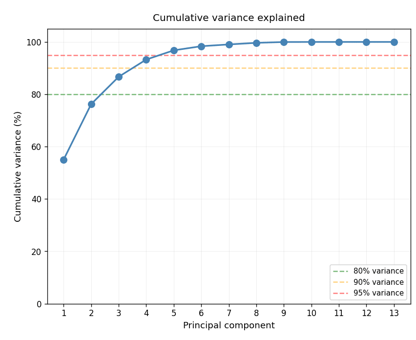
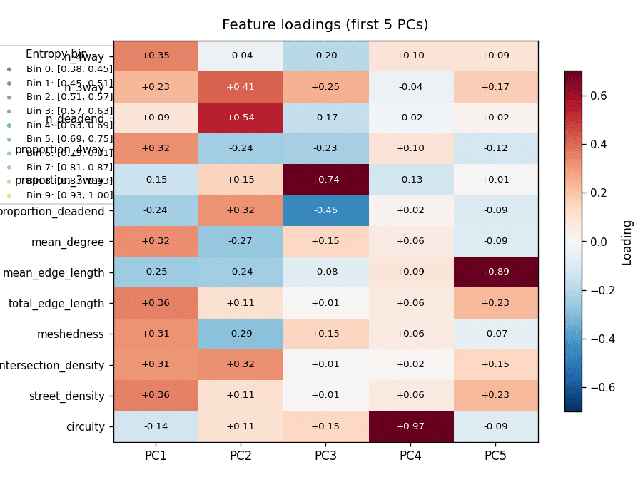
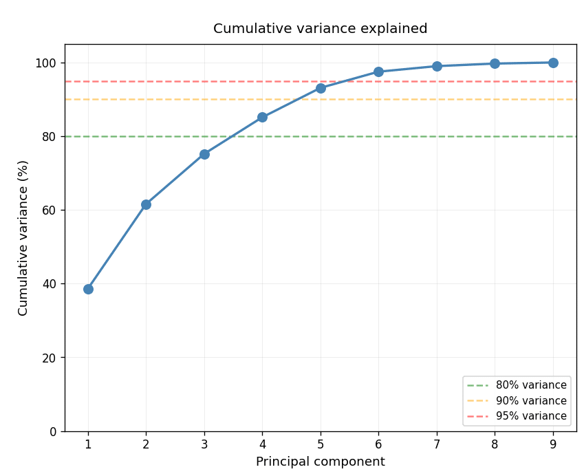
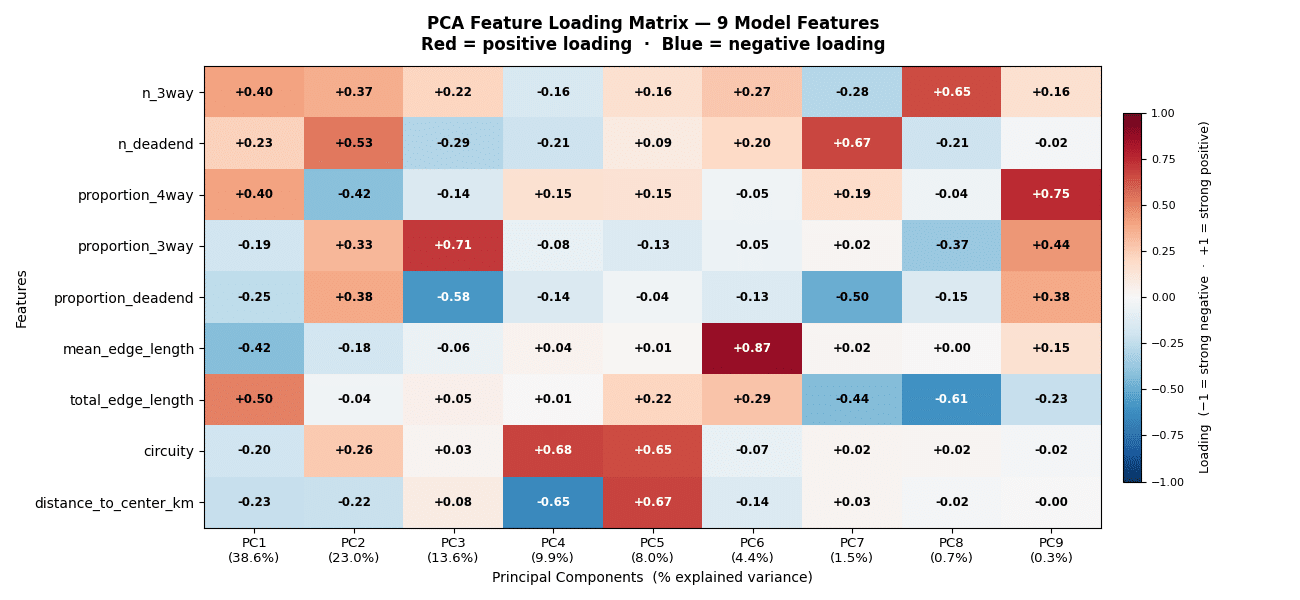
The correlation matrix exposed redundancy among grid-describing features such as mean degree, proportion of 4-way intersections, and total edge length. PCA reinforced this: PC1 alone captured nearly 50% of the variance, meaning the feature space carried less independent information than its dimensionality implied. Circuity and mean edge length stood out as genuinely independent.
PCA 01
PCA 02
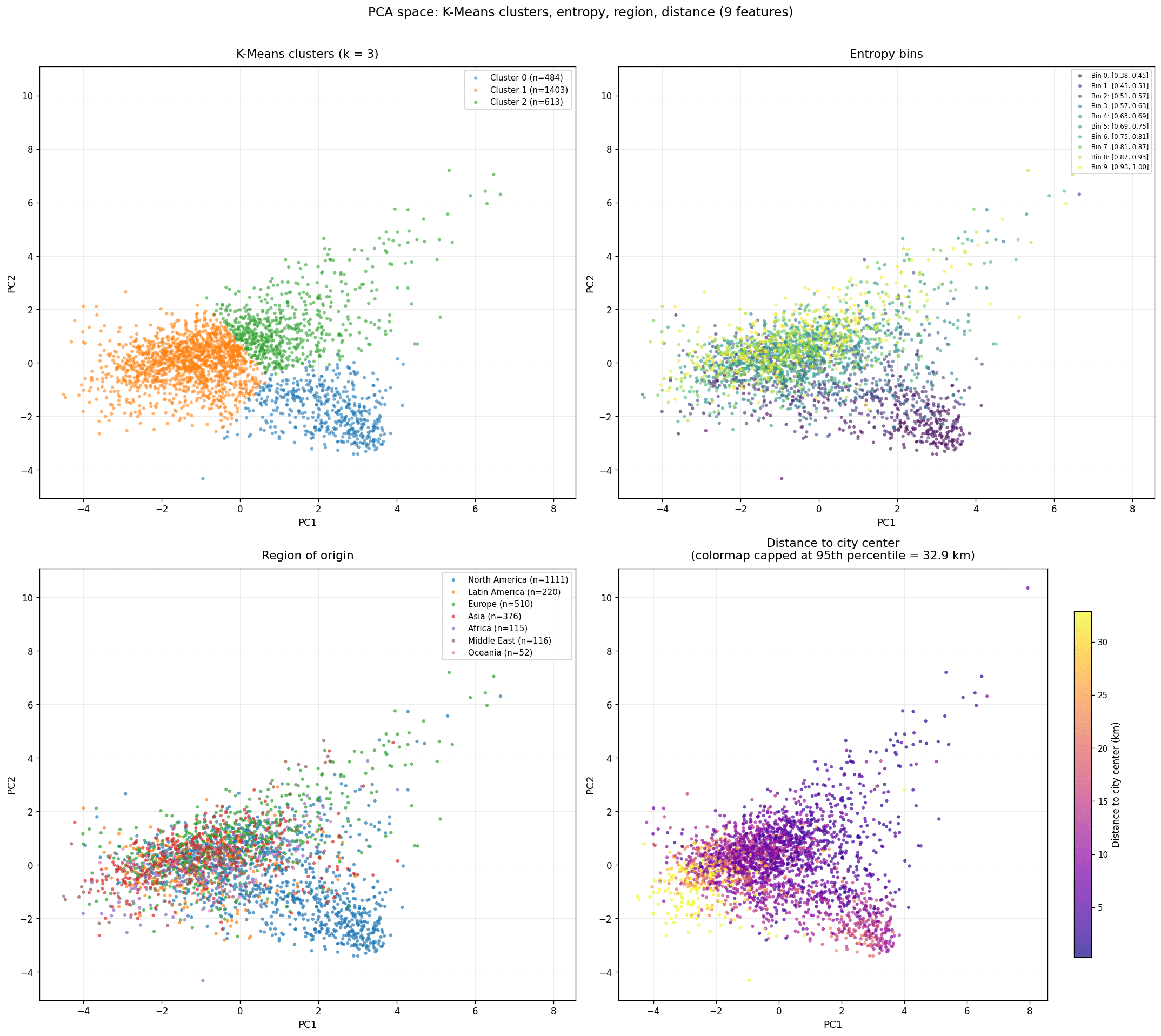
Acting on this, we dropped redundant features and added distance to city center. The updated PCA showed variance spread more evenly across components, a modest but real improvement, and surfaced a correlation between circuity and distance to center. Re-running K-Means, the 5-cluster solution was now less crisp; 3 clusters read cleanest, though the main distinguishing signal remained the North American low-entropy grouping.
K-means clustering 02

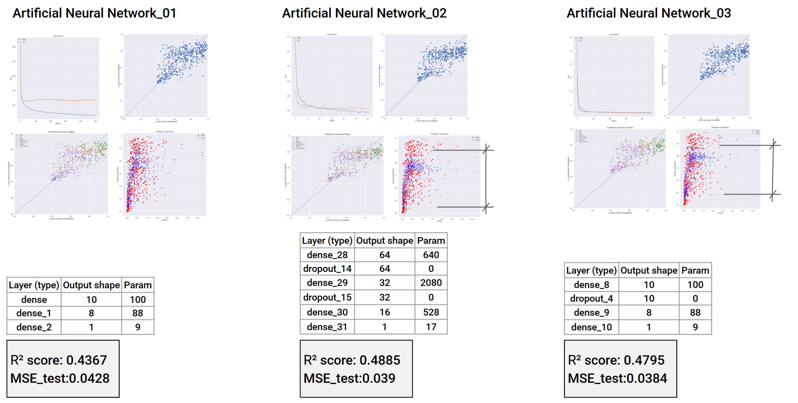
Model training
We trained a neural network, testing several architectures and settling on a deeper one that minimized squared error. The predictions compressed toward the middle of the entropy range, suggesting the model handles medium-entropy patches more confidently than the extremes, a known tension we’ll address next, likely with XGBoost and targeted handling of the distribution tails.
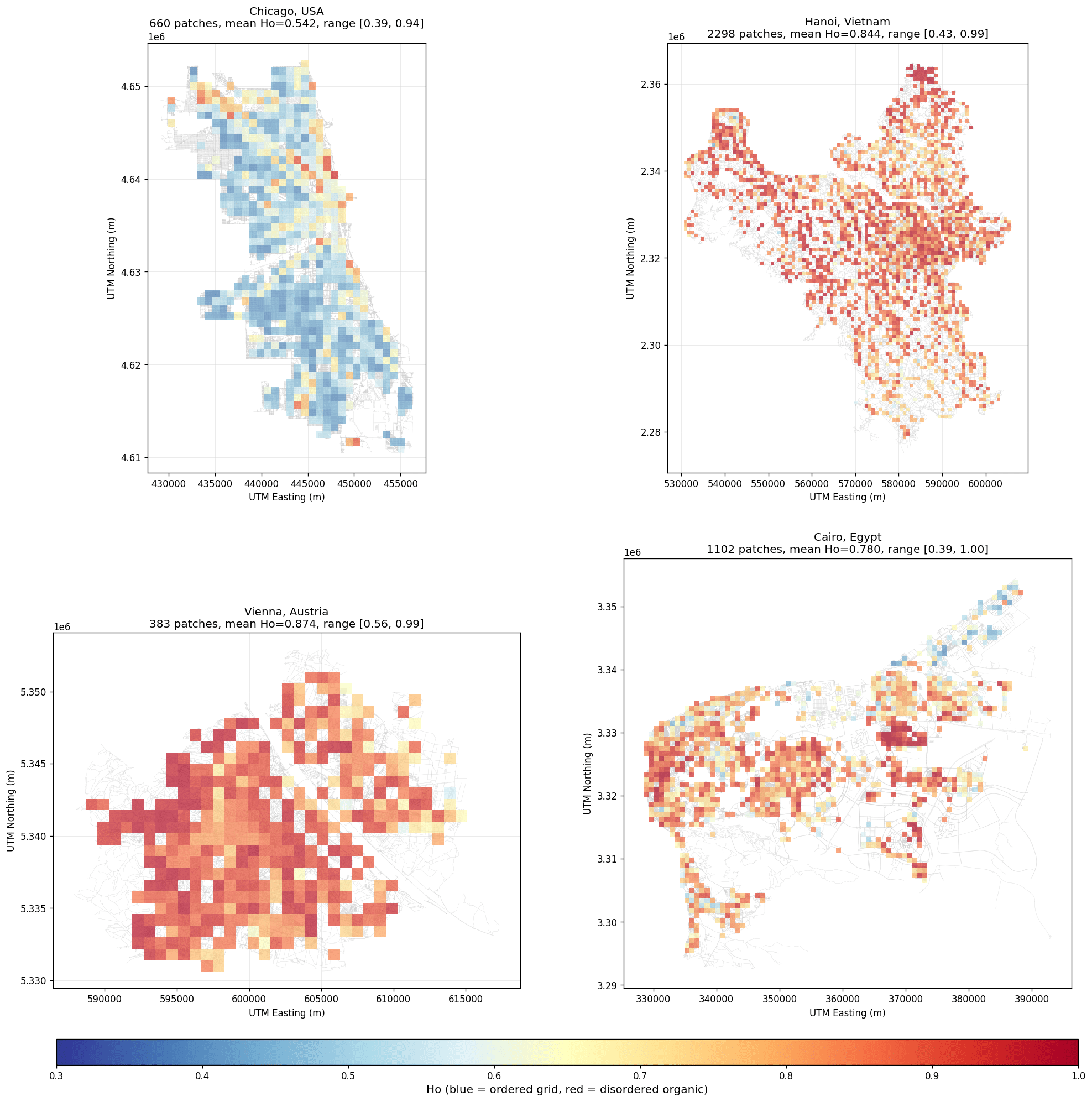
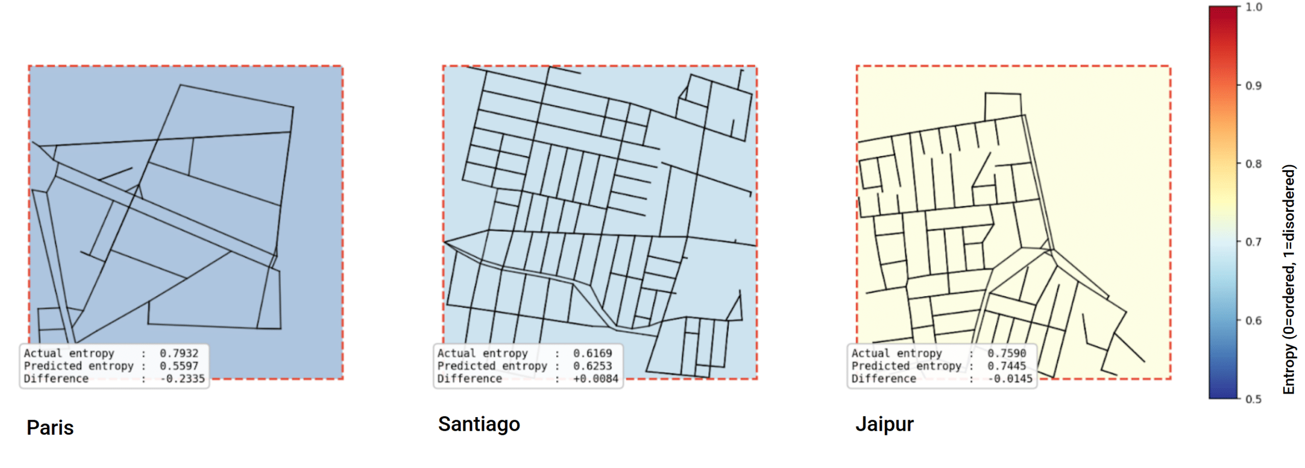
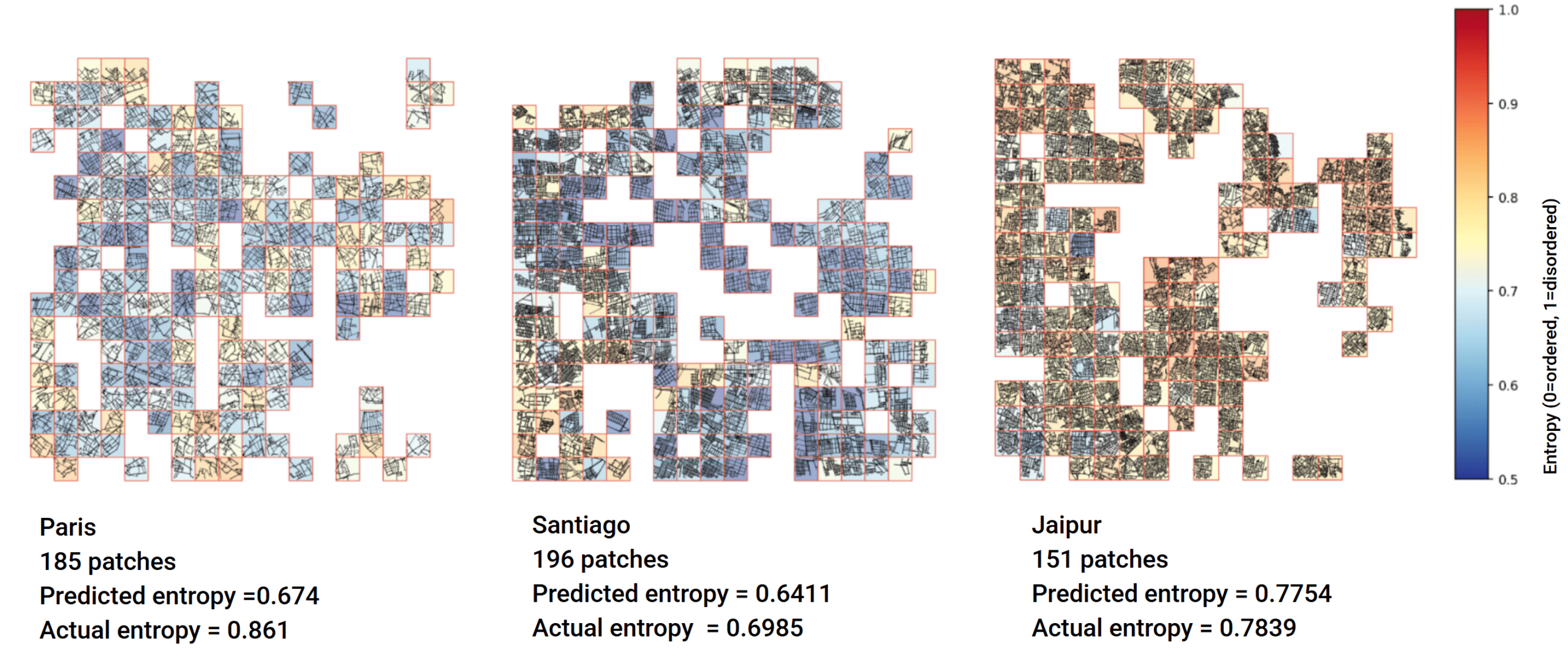
Deploying: from single patches to whole cities
We deployed the trained neural network at two scales: on individual patches and on entire cities. The most notable pattern was an accuracy gap tied to the underlying urban form. The model predicted entropy more accurately for cities with higher entropy, while struggling with more ordered, lower-entropy cities. The compression toward mid-range values we saw during training carried through to deployment, hitting the low-entropy end hardest.
What City-Level Deployment Revealed
Running predictions across a full city surfaced one of the most valuable insights of the project: a chance to sharpen our filtering logic.
At the start, we filtered patches using intersection count as a proxy for urban quality, discarding outskirts, parks, and industrial zones to capture each city’s true identity. Deployment showed this worked well for many European cities, where dense intersections coincide with the historic core, but revealed its limits for cities like those in Latin America, whose central character isn’t necessarily tied to intersection density. As a result, some city-center patches were filtered out, and the dataset leaned toward a particular kind of urban fabric.
This is exactly the kind of finding that only emerges once a model meets real cities at scale, and it points clearly to the next improvement: filtering on urban centrality rather than raw intersection counts. Centrality captures the structural importance of a location within the network, not just how many streets meet there, letting the dataset reflect each city on its own terms. It’s a natural next step, and one this deployment phase made obvious.