
A theory review of Chapter 18 of Russell & Norvig’s Artificial Intelligence: A Modern Approach
This chapter was assigned for the AIA Theory seminar at the beginning of the MaCAD 2025–2026 program, as part of a sequence of foundational readings on artificial intelligence. The seminar pairs canonical AI literature with discussion around its implications for design, knowledge production, and the assumptions embedded in computational systems.
Chapter 18 of Russell and Norvig — Learning from Examples — sits early in this sequence because it sets out the basic vocabulary of machine learning: what it means for an agent to learn, how learning problems are categorised, and the families of models used to solve them. The chapter is technical, but most of its concepts return throughout the rest of the master’s, in studio, in graph machine learning, in data encoding. Reading it once at the start gives a shared reference that the rest of the term can build on.
The review that follows is structured around the original chapter sections. Each part presents the key ideas alongside the figures Russell and Norvig use to illustrate them.
0. Introduction
An agent is learning if it improves its performance on a future task after making observations about the world.
There are three reasons to use machine learning instead of writing rules by hand:
- the designer cannot anticipate every possible situation the agent will face,
- the designer cannot anticipate every change over time, and
- in some cases there is no known way to program a solution directly.
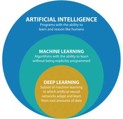
Machine learning sits inside the broader category of artificial intelligence — programs that learn and reason — and contains the narrower subset of deep learning, which relies on artificial neural networks trained on large quantities of data.
1. Forms of learning
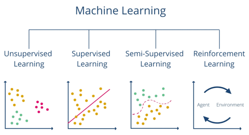
Learning can be classified by the type of feedback the agent receives.
In unsupervised learning, the agent looks for patterns in the input without explicit feedback. Clustering is the standard example.
In supervised learning, the agent is given example input–output pairs and learns a function that maps one to the other.
In semi-supervised learning, only a small portion of the data is labelled; the agent must use the rest of the unlabelled data to fill in the gaps.
In reinforcement learning, the agent learns from a series of rewards and punishments rather than from labelled examples.
Within supervised learning, the type of output divides the problem further: classification when the output is a finite set of values, regression when the output is a number.
2. Supervised Learning
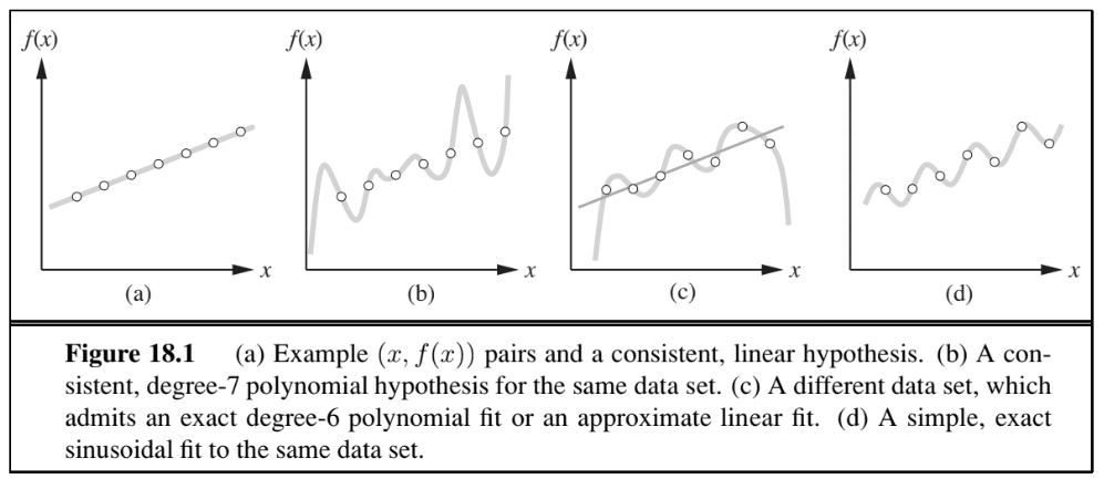
Given a training set of N input–output pairs, the task is to find a hypothesis h that approximates the true function f.
The accuracy of h is measured against a test set that is kept separate from the training data. We say h generalises well if it predicts y correctly for examples it has not seen before.
When multiple hypotheses fit the data equally well, Ockham’s razor suggests choosing the simplest.
3. Learning decision trees
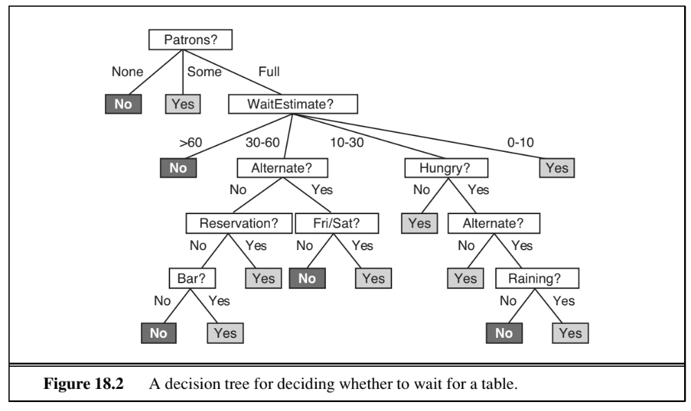
A decision tree takes a vector of attribute values as input and routes it through a sequence of tests, returning a single definitive answer.
The standard learning algorithm uses a greedy divide-and-conquer strategy: at each node, it splits on the attribute that makes the most difference for classification, aiming to minimise the depth of the final tree.
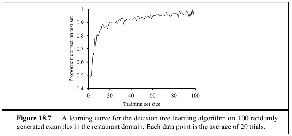
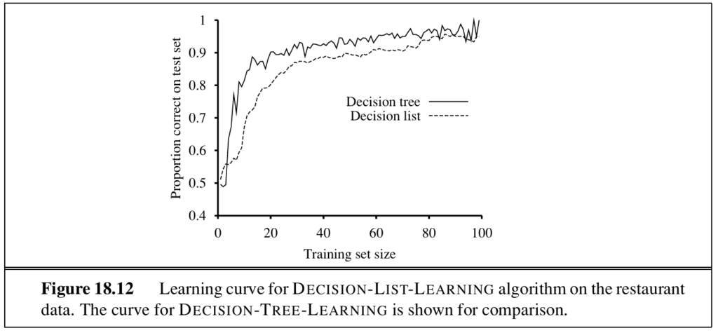
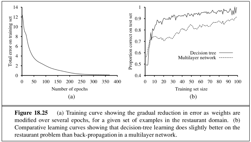
The performance of the algorithm is measured by the learning curve, which plots accuracy on the test set as a function of training-set size.
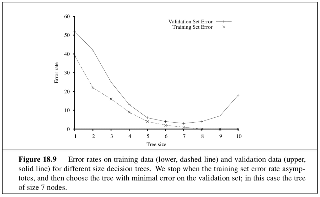
Overfitting occurs when a model reaches very high accuracy on the training set but fails to generalise. Decision-tree pruning removes nodes that are not clearly relevant and is the standard remedy.
4. Choosing the best hypothesis
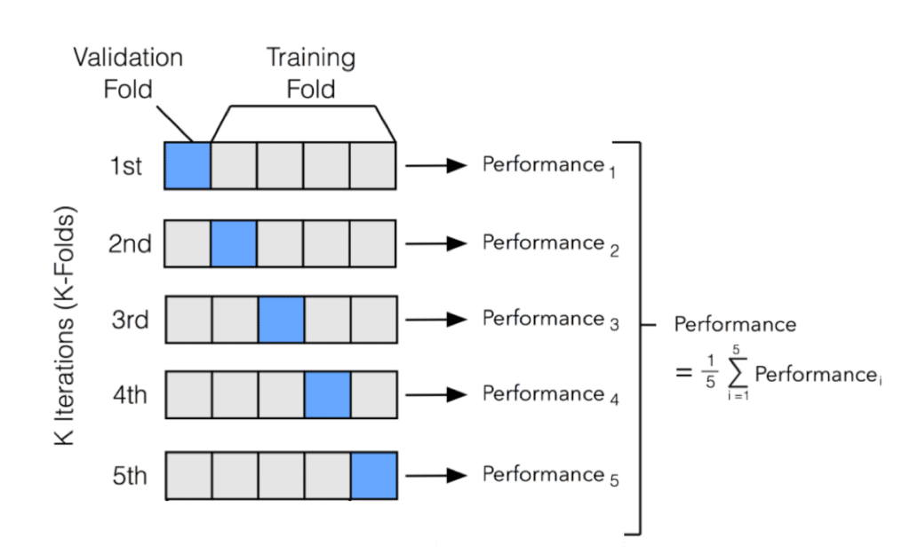
Cross-validation is a statistical method for assessing how well a model generalises to an unseen dataset. The most common variant is k-fold cross-validation, where the dataset is split into k equal folds and each fold serves as the test set exactly once.
A validation set is a subset of the training data used to measure performance during training, separate from the final test set.
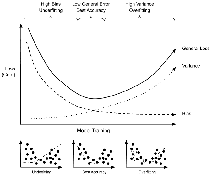
Model selection defines the hypothesis space; optimisation then finds the best hypothesis within it. An algorithm that performs both is a wrapper — it takes the learning algorithm as an argument. The usual procedure starts with the simplest model, which probably underfits, and increases complexity step by step until the models start to overfit.
The error rate of a hypothesis is the proportion of mistakes it makes. A loss function quantifies how bad each error is, measuring the utility lost. The total cost is the weighted sum of empirical loss and the complexity of the hypothesis.
5. The theory of learning
Computational learning theory is based on the principle of the probably approximately correct (PAC) hypothesis. A PAC learning algorithm is one that returns a hypothesis with a small bounded error rate, with high probability.
Decision lists are an example. They resemble decision trees but branch in only one direction.
6. Linear models
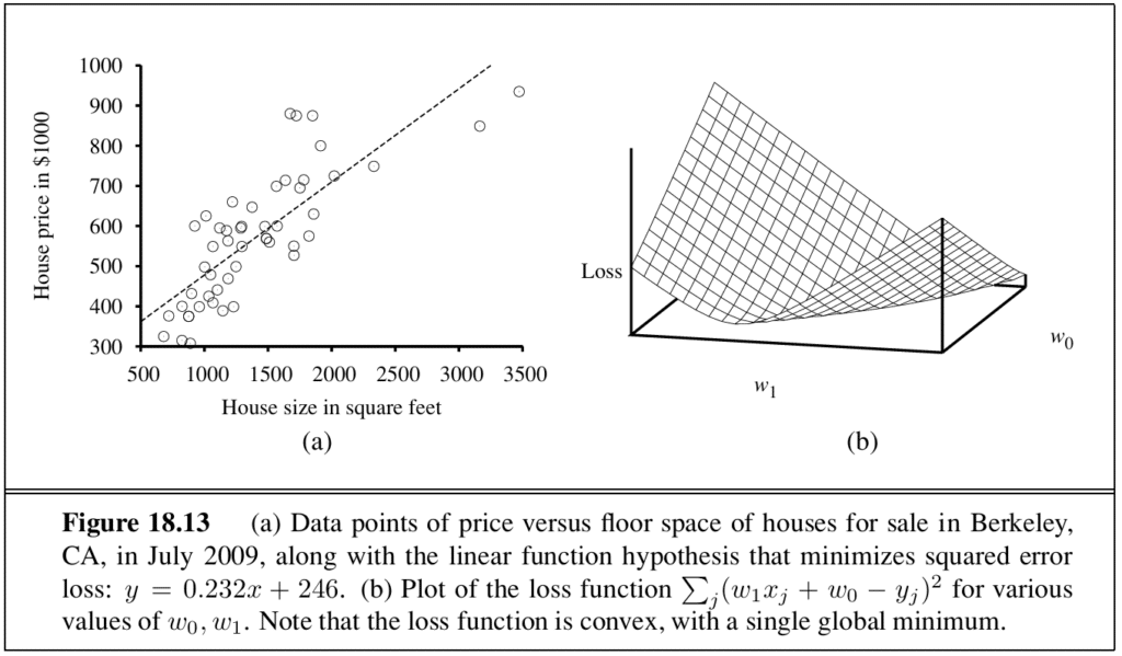
Univariate linear regression consists of finding the function
h_w(x) = w₁x + w₀
that best fits the dataset — that is, finding the weights that minimise the empirical loss. The standard choice is the squared loss function L₂, which is convex and has a single global minimum.
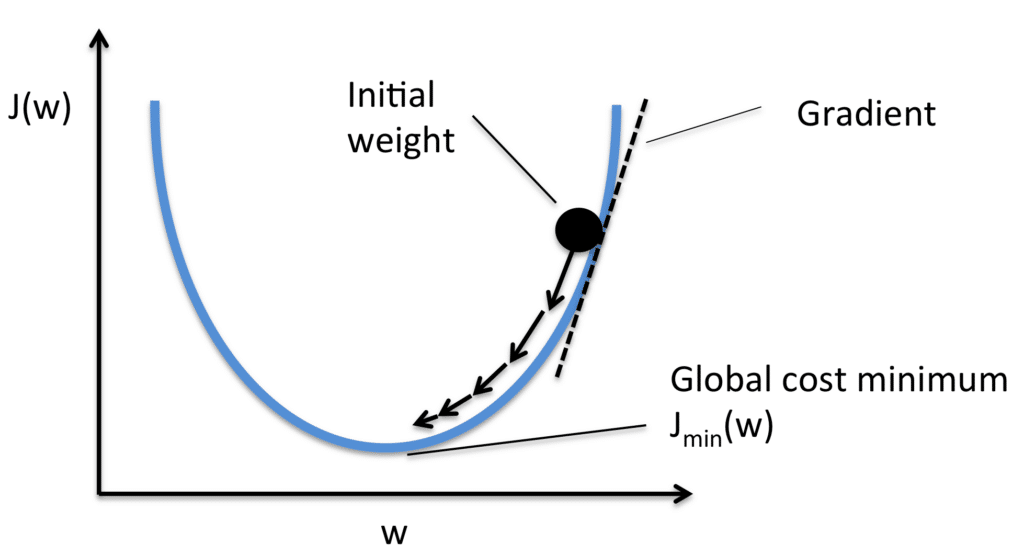
When the loss equations have no closed-form solution but a continuous weight space, the solution is found through gradient descent: a hill-climbing algorithm that follows the gradient of the function being optimised. The step size is called the learning rate.
In multivariate linear regression, the hypothesis takes the form
h_w(x_j) = w₀ + w₁x_{j,1} + ⋯ + w_n x_{j,n}
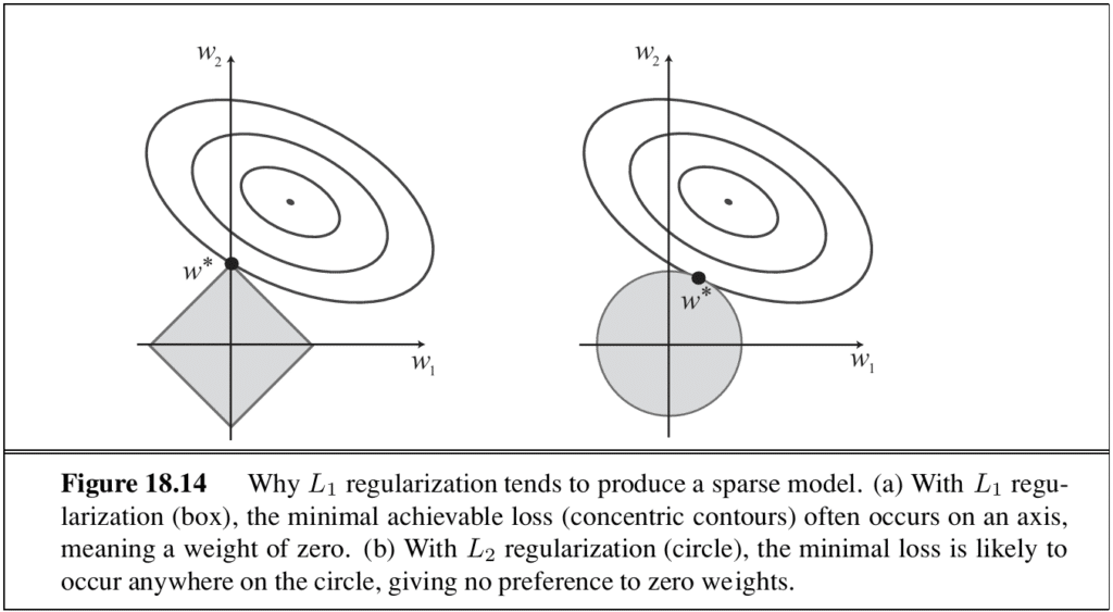
The intercept w₀ can be multiplied by a dummy input x_{j,0} = 1. Regularisation avoids overfitting by minimising total cost; L₁ regularisation has the further advantage of producing a sparse model by setting many weights to zero.
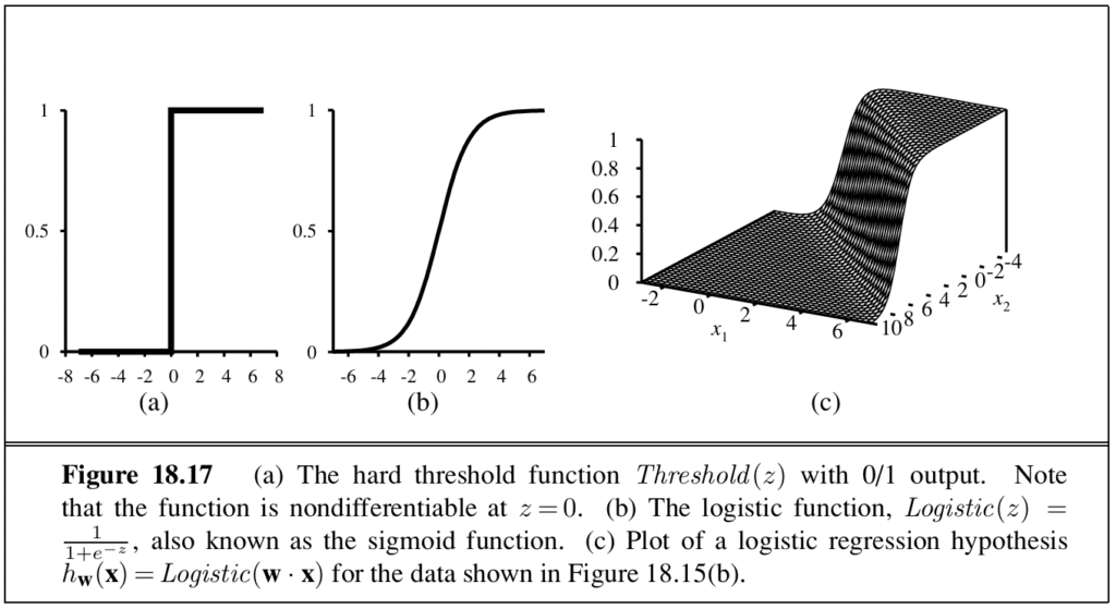
A linear classifier is produced by passing a linear function through a threshold. With a hard threshold — a perceptron — the classifier can be trained by a simple weight update rule, but only on linearly separable data. For noisy or non-separable data, logistic regression replaces the hard threshold with a soft one defined by a logistic function.
7. Artificial neural networks
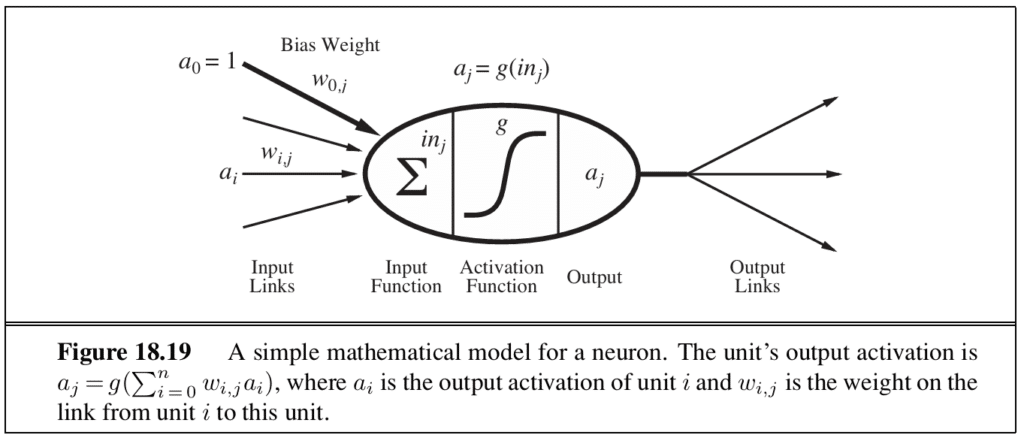
Neural networks mimic the electrochemical activity in networks of brain cells. They are composed of linear-threshold units connected by links that propagate activation. Each link carries a numeric weight that determines the strength and sign of the connection. The networks can represent complex nonlinear functions.
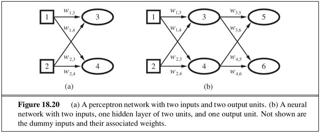
Feed-forward networks are organised in layers, with each unit receiving input only from the immediately preceding layer. They are called single-layer (perceptron) when they contain only input and output layers, and multilayer when they include hidden layers between the two. The number and size of hidden layers is determined through cross-validation.
Neural networks are, in essence, a tool for nonlinear regression. The back-propagation algorithm implements gradient descent in parameter space to minimise the output error.
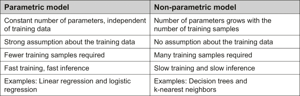
8. Nonparametric models
Nonparametric models use all the data to make each prediction, rather than summarising the data first with a small set of parameters. Nearest-neighbour methods and locally weighted regression are the standard examples.
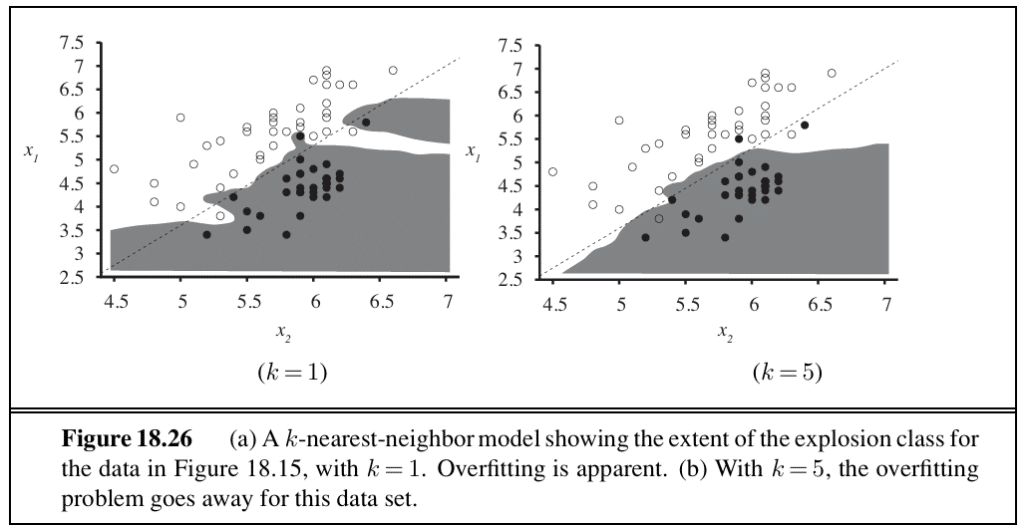
k-nearest neighbours improves on a lookup table with a small variation: given a query point x_q, find the k examples that are nearest to x_q. Methods for finding nearest neighbours include the k-d tree — a balanced binary tree with arbitrary dimensions — and locality-sensitive hashing, which returns an approximate solution faster.
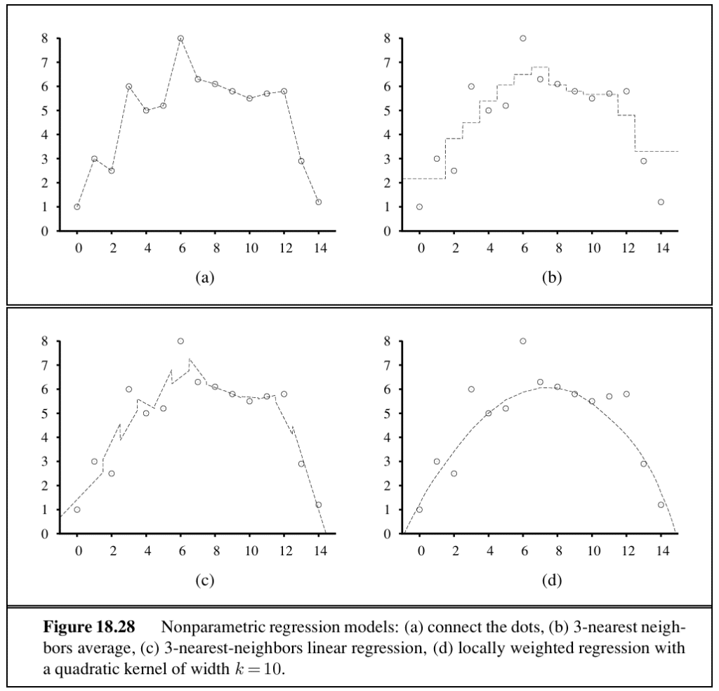
Locally weighted regression is the nonparametric model that tends to generalise best. It weighs the training examples by their distance to x_q using a function called a kernel, which is itself chosen by cross-validation.
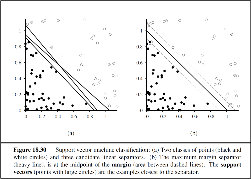
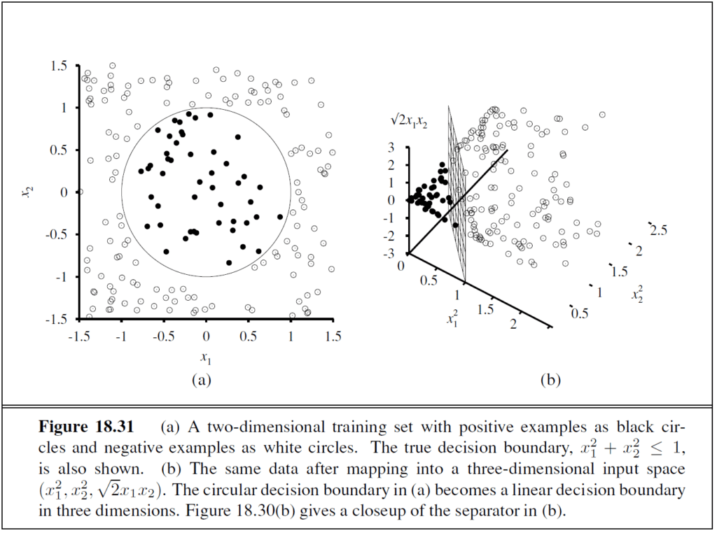
9. Support vector machines
Support vector machines (SVMs) find linear separators with the maximum margin between classes, which improves the classifier’s generalisation performance. Kernel methods implicitly transform the input data into a high-dimensional space where a linear separator may exist, even when the original data are not separable.
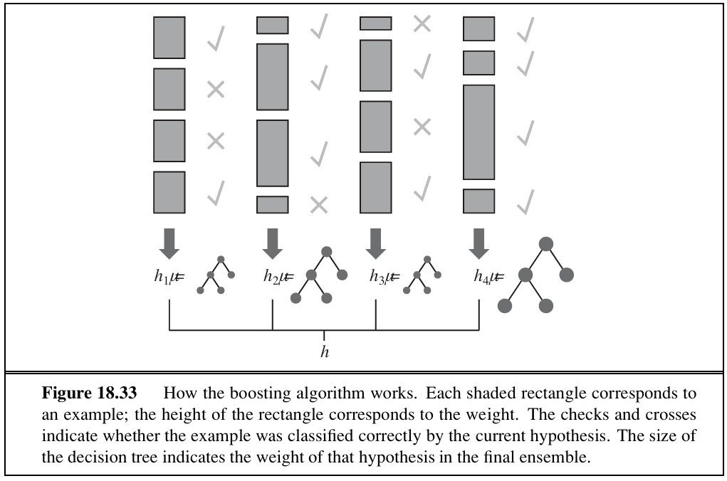
10. Ensemble learning
Ensemble methods select a collection of hypotheses from the hypothesis space and combine their predictions. They often perform better than any individual method.
The most widely used is boosting, which trains successive models on a weighted version of the training set. In online learning, the predictions of multiple experts can be aggregated so that the combined model performs arbitrarily close to the best individual expert, even when the data distribution shifts over time.
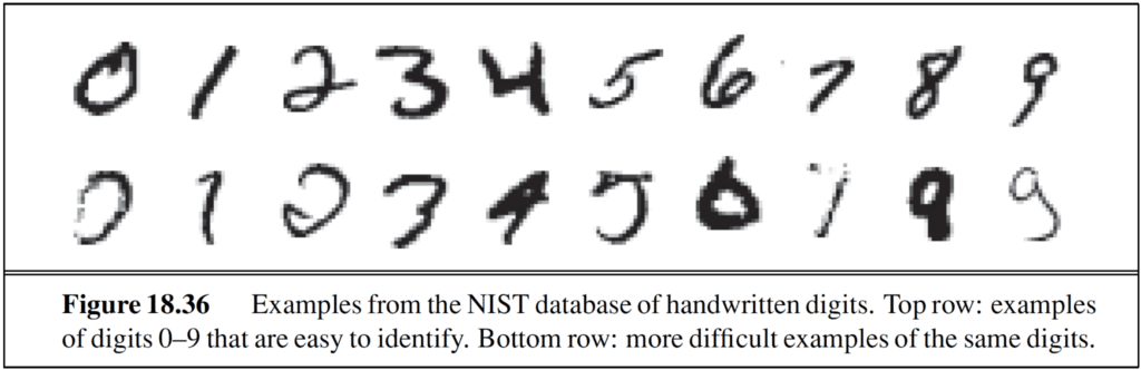
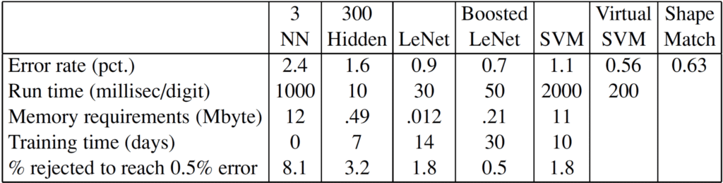
11. Practical machine learning
In practice, machine learning prioritises data over algorithmic complexity. Better algorithms have, for instance, improved handwriting recognition to near-human accuracy, but increases in training-data volume usually yield larger performance gains than improvements to the model.
Real-world success depends heavily on feature engineering — the selection of the most predictive variables from the available data.
Selected exercises
A few exercises were worked through in the seminar to test the concepts introduced in the chapter.
Exercise 18.2 — The football player
Consider the problem faced by a football player learning to play football. Explain how this process fits into the general learning model. Describe the percepts and actions, the types of learning involved, and the subfunctions the player is trying to learn in terms of inputs, outputs, and available example data.
Football players learn through two principal mechanisms. The first is reinforcement learning: match outcomes such as scoring or losing possession act as rewards or punishments, gradually refining decision-making over many games. The second is supervised learning: coaches provide explicit, labelled instructions on the correct move for specific scenarios. In practice players blend the two — mastering coached drills while using trial-and-error to adapt to the unpredictable flow of a game.
Exercise 18.3 — Recovering a decision tree
If you generate a training set from a specific decision tree and then apply the decision-tree learning algorithm to that data, will it return the correct tree as the data approaches infinity?
Given infinite data, a fully consistent and unrestricted learner can recover the original decision tree, or a logically equivalent simpler one. Standard algorithms such as ID3, C4.5 and CART do not guarantee this, however. Their greedy splits, pruning rules and tie-breaking can lead them to converge on a structurally different tree that still represents the same function.
Exercise 18.11 — The majority classifier
A dataset has 100 positive and 100 negative examples. Using leave-one-out cross-validation, the majority classifier scores zero every time. Explain why.
If a positive example is chosen as the test point, the remaining training set contains 99 positive and 100 negative examples — so the majority is negative and the classifier predicts negative. The test example was positive: wrong. If a negative example is chosen as the test point, the remaining set contains 100 positive and 99 negative examples — majority positive, prediction positive, actual negative: wrong again. Every prediction is incorrect.
Summary
Congratulations, you’ve read this far! 🎉
This text might look too technical at a glance, but so is Machine Learning – it is just math after all. It is not shiny or eye-catching, but you can see its beauty if you look closer.
Our summary of Chapter 18 was prepared at the very beginning of the AIA Theory seminar, and our understanding of the topic has developed as we have had the chance to test this theory in practice. Perhaps the biggest shift in our understanding was in the importance of data itself. The core concepts of how the magical black box works in the background have to be understood, but from what we have learnt so far, it is the data work – scraping, preparation, cleaning, and the endless attempts to plot each variable in the hope of understanding what the dataset actually consists of and how it behaves – that turns out to be the most crucial part of the whole process. Oh, and also, defining what we are actually trying to predict! And always remembering to ask ourselves whether machine learning is needed for that purpose at all. After all – it is us, humans, who lead the process.
