
What is an isovist?
Isovist analysis helps architects and designers understand how people perceive and navigate through spaces, enabling them
to optimize layouts, enhance wayfinding, and create more engaging and functional environments.
This project has only work over the isovist area calculation, in which the final isofield image represents each of the points of view visible areas in a black to white colormap.
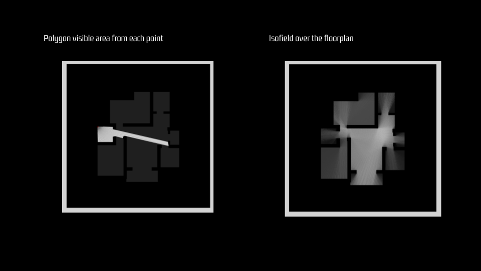
Circularity = (4? * Area) / (Perimeter^2)

Although the most common analysis are based in the isovist polygon area, there are multiple isofield interpretations like “Circularity”, where higher values indicates circular shape vision, and lower values indicate more irregular fields of view for the observer.
Why?
Architectural and urban design processes require iterative solutions, coupling analysis and modeling tools to facilitate the workflow. Integration of analysis methods into the modeling process allows for real-time evaluation, minimizing interruptions and speeding up calculations for immediate feedback.
On average, isofield algorithms take approximately 2-3 seconds to update any geometric change in an floorplan of 80m2, making it very inconvenient for designers.
Objective
Train a generative neural network able to generate the images of an isovist calculation in almost real time, trying to overpass the geometric calculation times.
Methodology:
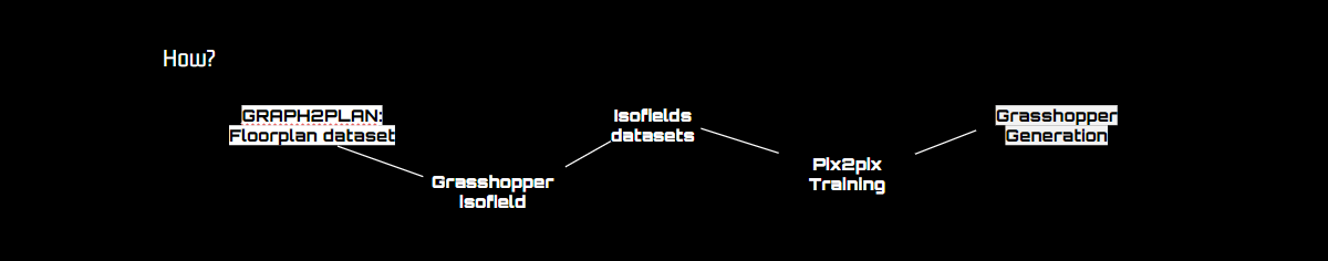
1.0. Source Dataset
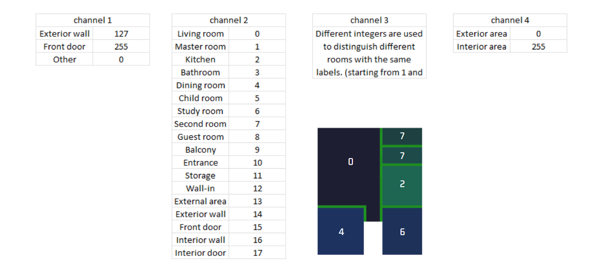

The mean values of each property is adequate for the room utility, besides all samples are showing a realistic gaussian distribution.
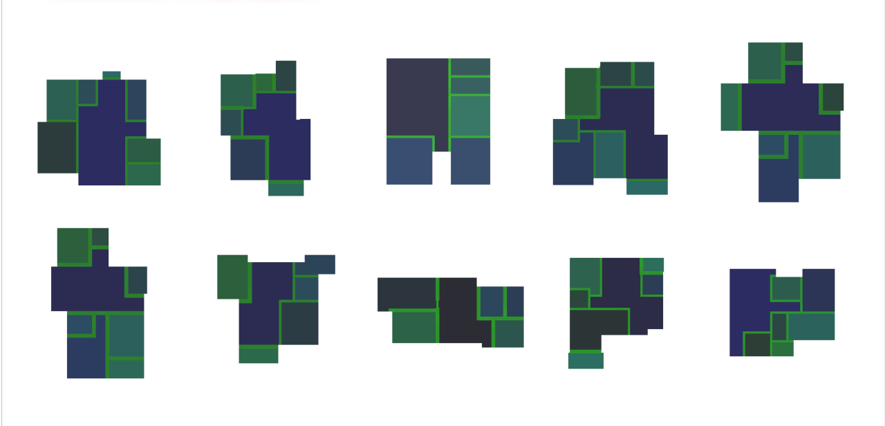
1.1. Obstacles dataset
The resulting training input dataset created is composed by two pixel values: obstacle=0, empty=255. The floor plans are constrain square boundary of to a 25.6×25.6m, which means every pixel represents 0.10m.
1.2. New isovists datasets
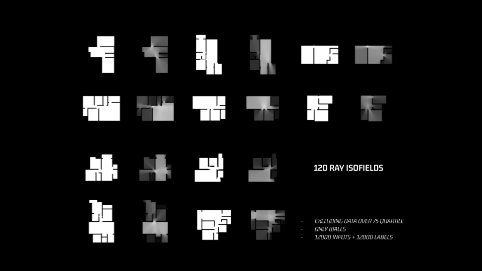
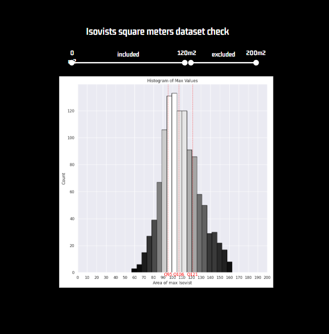
The new target dataset is a colormap based in a linear relation from 0-120m2 to 0-255rgb. For this, the training dataset excluded any samples over 120m2 of maximum polygon calculated with the objective of not presenting outliers values to the generative model.

2. Evaluation of dataset
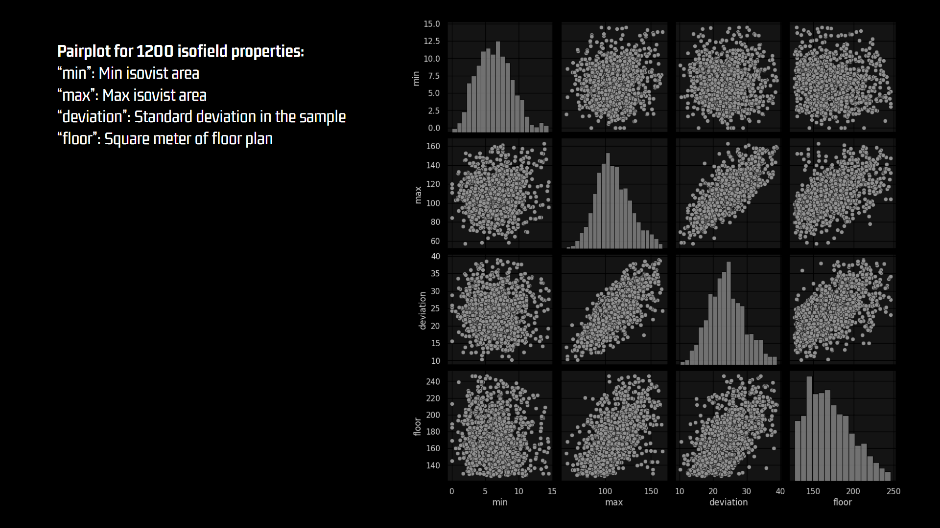
- floor-max: Good correlation between the maximum visivle area obtained in the floor plan and the total area of same floor plan.
- deviation-max: Good correlation between the maximum visivle area obtained in the floor plan and the mean deviation of maximum and minimum visible areas of same floor plan.
3. Training
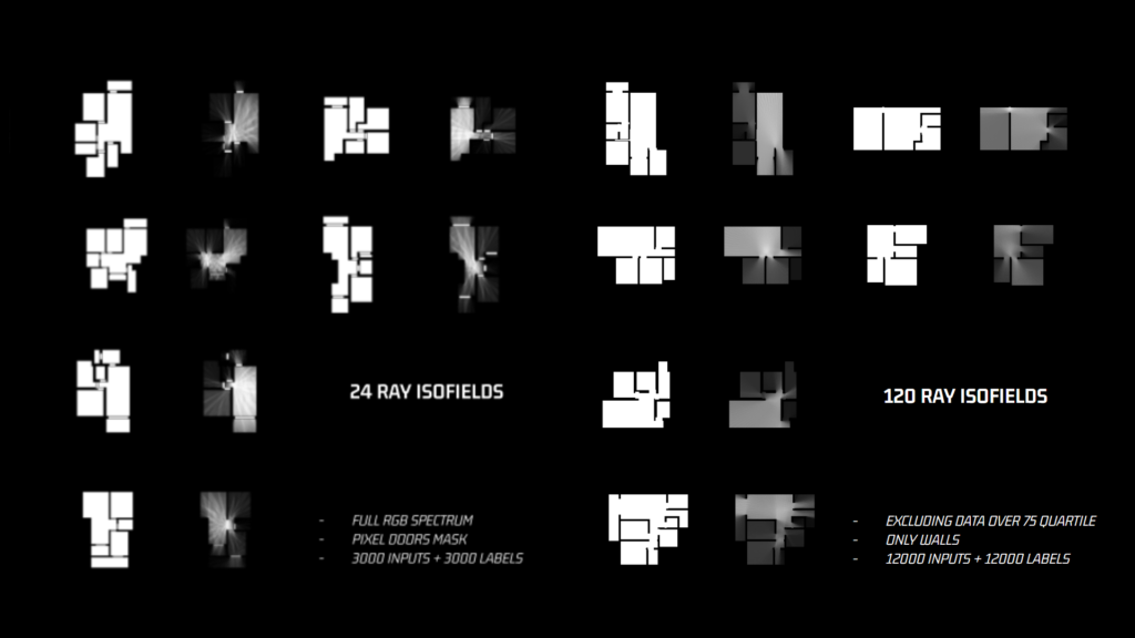
For the best performance of the pix2pix model, two datasets were produced and tested:
24 rays calculation and 120 rays calculation
first one more rough for the area estimation, but easier to understand the visual connections.
second one more soft, costly to produce and precise but not so much helpful for discerning areas.
Pix2Pix model:
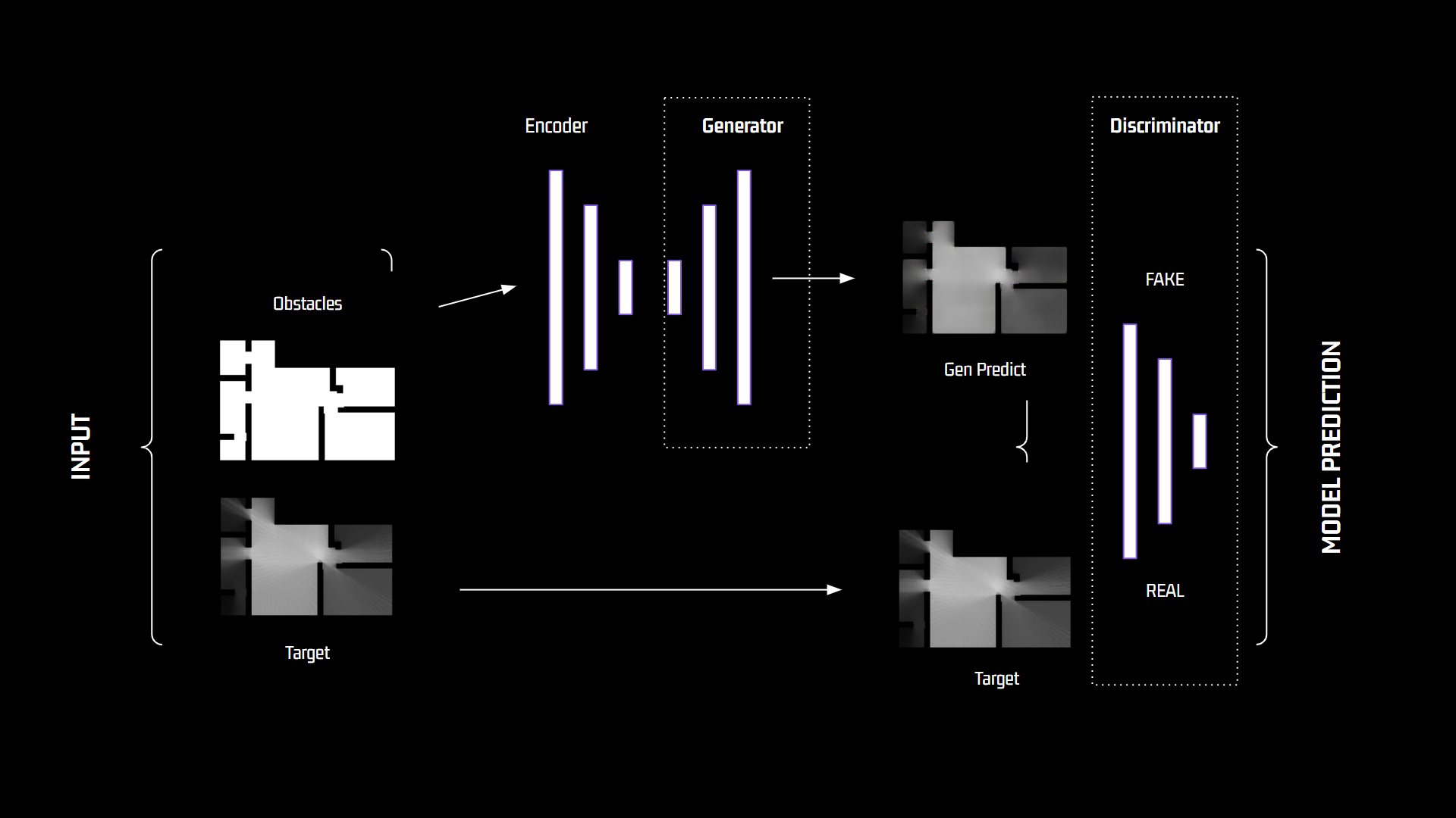
In a pix2pix model, there are two main CNNs models working together in an adversarial manner.
The generator is responsible for generating synthetic images based on random noise or other input representations, in this case from the blank floor plan input. The discriminator is trained to compare the real isovist image with the one generated by generator in a scoring system until outputs are indistinguishable.
3.1. 24RAY training batch
- Image size: 256 x 256 pix
- Kernel size: 4
- Training epochs: 8000
- Doors and walls as obstacles
- 24ray polygons
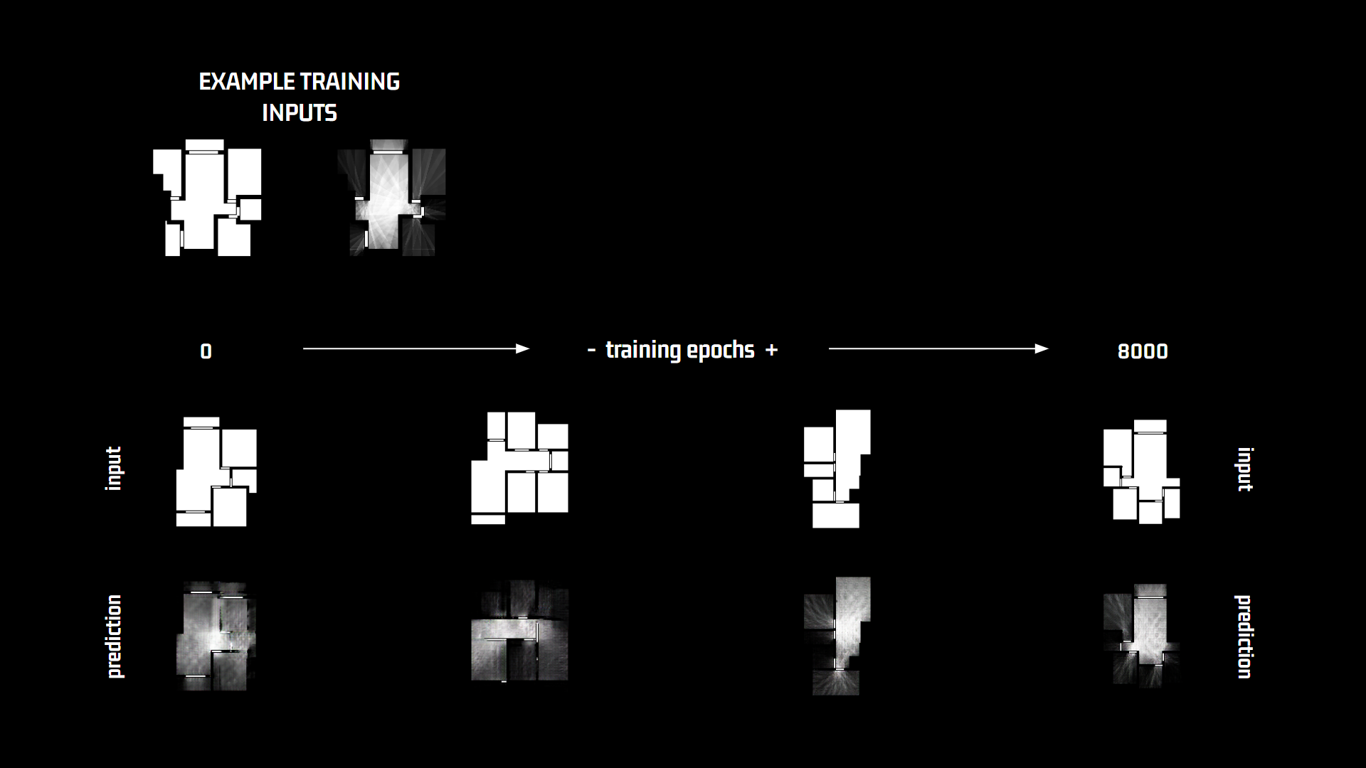
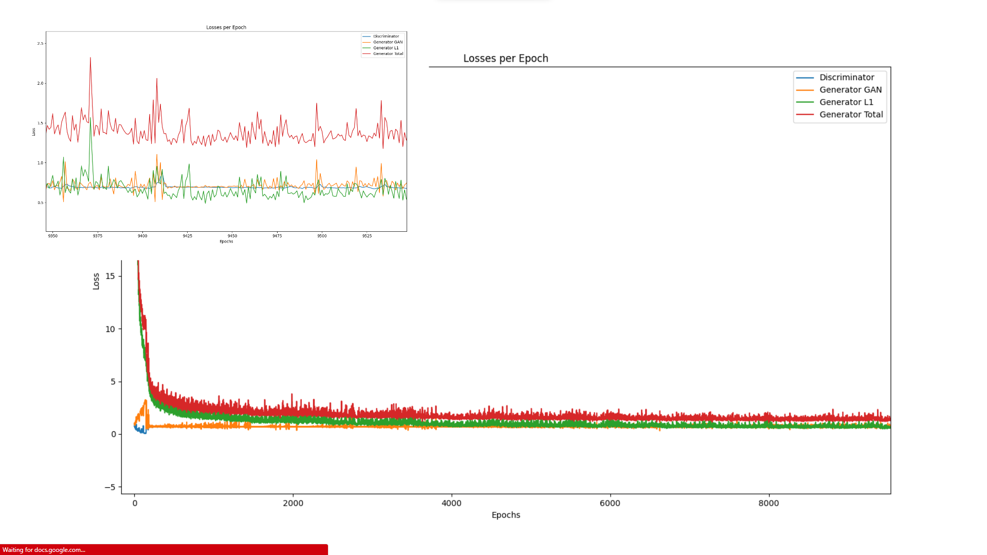
This first trial with the low resolution isovists was trained up to 8000 epochs and stopped with a “total generator loss” of 1.6
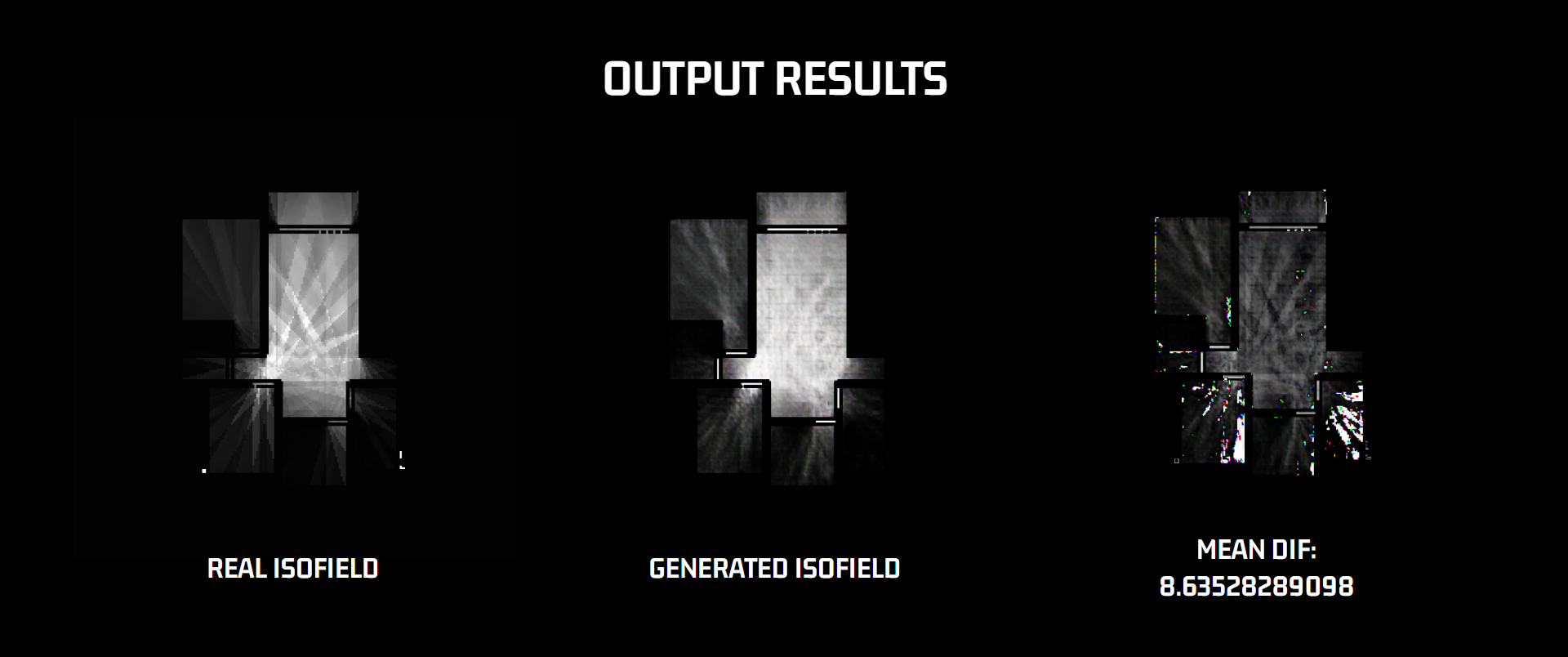
The absolute difference of pixels real/generated was 8.635 with maximums of 184 over 255. This maximum differences are represented on the right image in the white corners where the generator had more difficulties to fake the calculations.
For next test, doors representation was simplified and a more resolution isofields were created to ease the learning of the hard edges coming from the rays of views.
3.2. 120RAY training batch
- Image size: 256 x 256 pix
- Kernel size: 4
- Training epochs: 8000
- Walls obstacle
- 120ray polygons

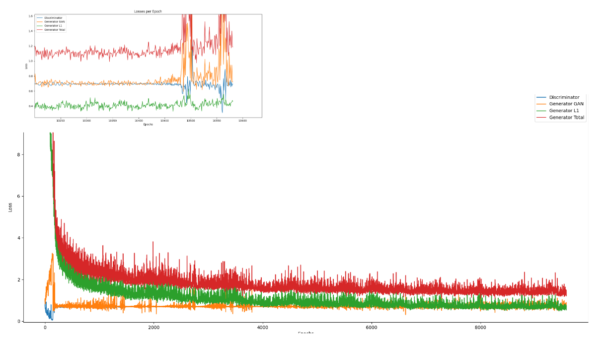
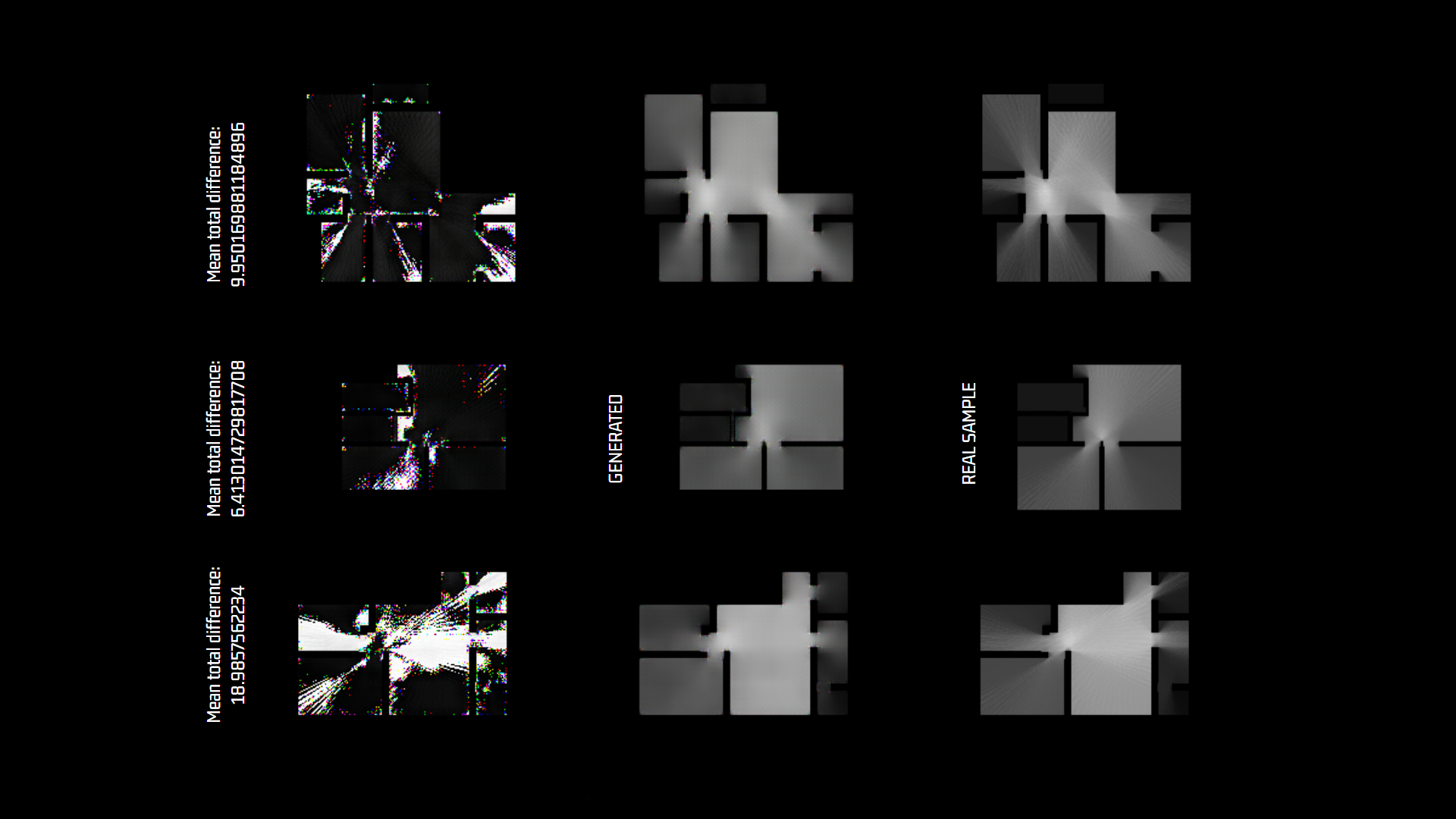
This second trial of high resolution obtained with a “total generator loss” of 1.2 after 8000 epoch, 0.5 lower result of the losses for both generator and discriminator scores.
The absolute difference of pixels real/generated was around 6 to 10 in most of the evaluated samples except for bad predictions of very large isovists with total differences of more than 18. This maximum differences are represented on the left image in the white corners where the generator had more difficulties to catch the prediction.
4. Grasshopper deploy
The model was deployed locally for real time floor plans analysis.
1. draw one single boundary curve representing all limits of floor plan
2. the updated boundary image is saved to the model training folder
3. the model outputs the prediction
4. grasshopper reads the image to show in the model space

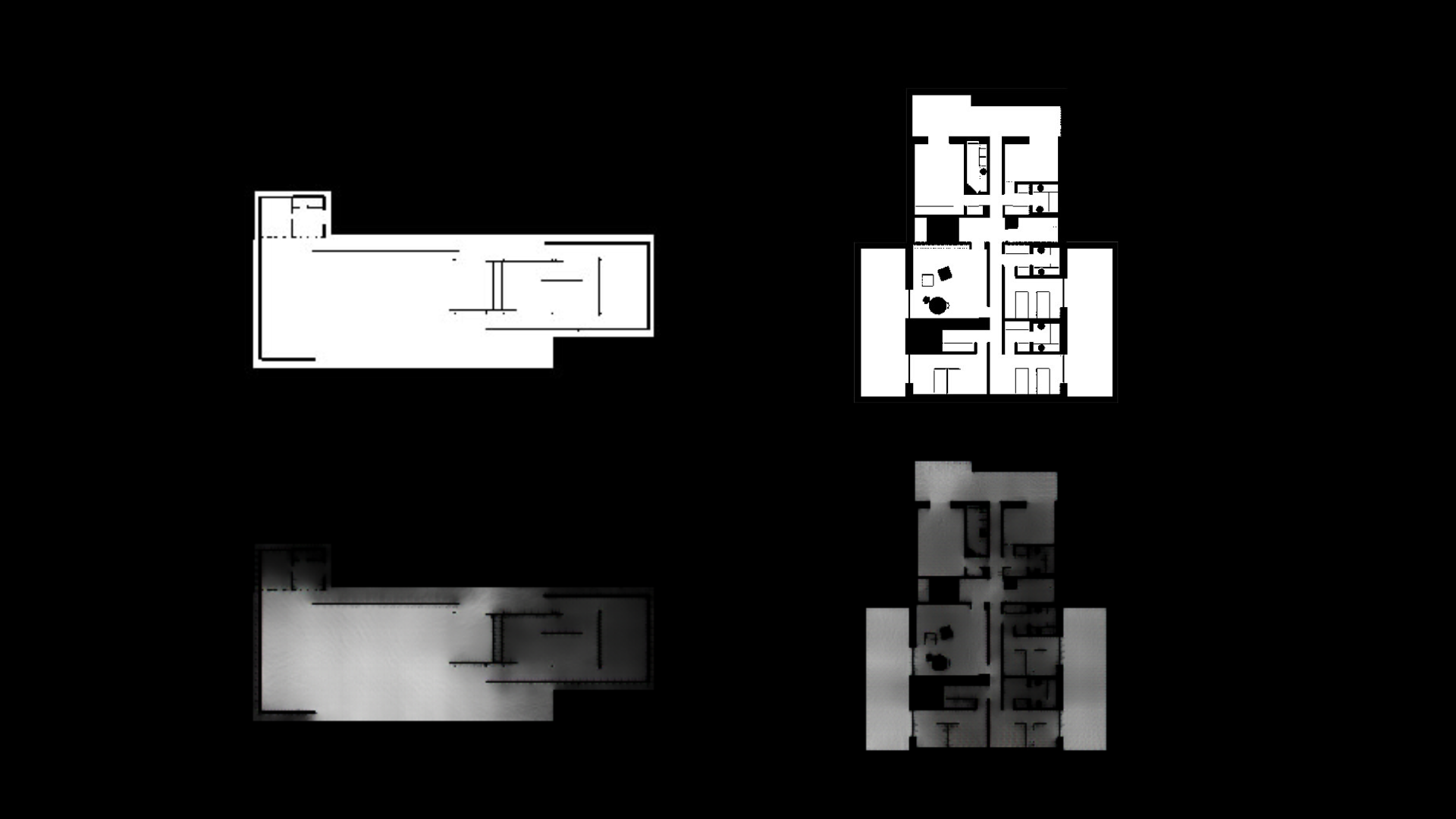
On the left, the the Barcelona pavilion from Mies van der Rohe, on the right, the Rau plan house from Alberto Campobaeza.
References:
- “StressGAN: A Generative Deep Learning Model for 2D Stress Distribution Prediction”
https://arxiv.org/abs/2006.11376 - “Real-Time Visibility Analysis – Enhancing calculation speed of isovists and isovist-fields using the GPU”
https://www.researchgate.net/publication/256471427_Real-Time_Visibility_Analysis_-_Enhancing_calculation_speed_of_isovists_and_isovist-fields_using_the_GPU
