
Introduction
According to the World Health Organization, around 1.19 million people die each year due to traffic accidents, and another 20 to 50 million suffer non-fatal injuries, many of which result in disability. Beyond the human toll, the economic costs related to treatment and care for those involved in traffic accidents are significant, estimated to be around 3% of the GDP for most countries.
Typically, traffic accidents are attributed to four main factors:
- Human behavior
- Vehicle efficiency
- Environmental conditions
- Infrastructure characteristics
However, there is another critical aspect that we, as professionals in urban design, have the power to influence: urban morphology. Urban morphology is vital because it shapes the interaction between all other factors. By altering the geometry of urban spaces, we can potentially reduce the number of traffic accidents.
To leverage urban design in reducing road incidents, it is crucial to understand the relationship between urban morphology and the frequency of accidents, as well as the strength of this correlation. In this project, we utilize digital tools such as Grasshopper, Hops, Python, and basic machine learning algorithms to create a pipeline which abstracts crash data and urban morphology features into encoded images, which are then plotted on a 2D plane to visualize their relationships.
Methodology
To visualize and better understand the relationship between urban morphology and traffic accidents, we designed a flexible and general pipeline that allows for experimentation with both the features of the spatial context being analyzed and the parameters chosen to train the AI models. The structure of the pipeline is divided into two stages: the construction of the dataset, and the training of the models followed by the visualization of the outputs.
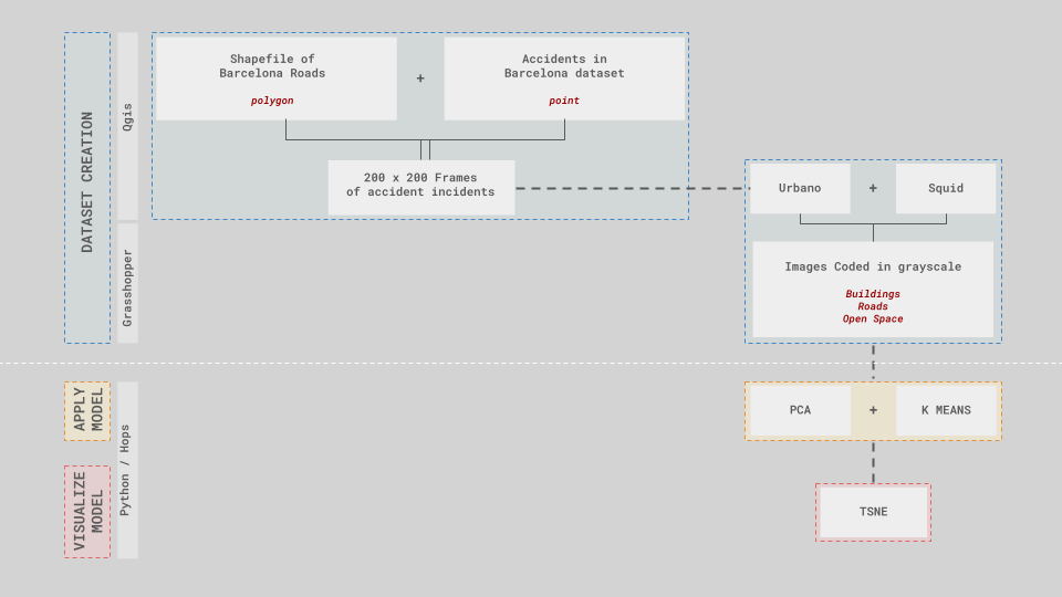
Dataset Construction
In the first stage of the pipeline, information about urban morphology is extracted and converted into images that can be read by ML models. The city of Barcelona was selected to generate the sample images due to the availability of data for both the urban context and traffic accidents.
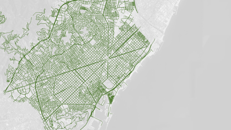
We start by examining the road network, which facilitates different mobility patterns. This step is crucial for proving the hypothesis that urban morphology and accidents are related, as the road network indicates the freedom and restriction of movement for vehicles and pedestrians.
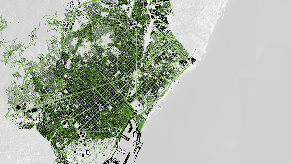
Next, we incorporate the immediate context of the roads, including buildings, crosswalks, traffic signs, traffic lights, and more. This context significantly affects visibility and sight lines for pedestrians and drivers, vehicle speeds, pedestrian movement patterns, and various other behaviors. This data is subject to variation; adding or omitting certain contextual elements can positively or negatively impact the dataset, making the relationship to the number of incidents either more cohesive or noisier.
Finally, after gathering all contextual information, we add the frequency of road accidents to compare different morphologies by their accident proneness.
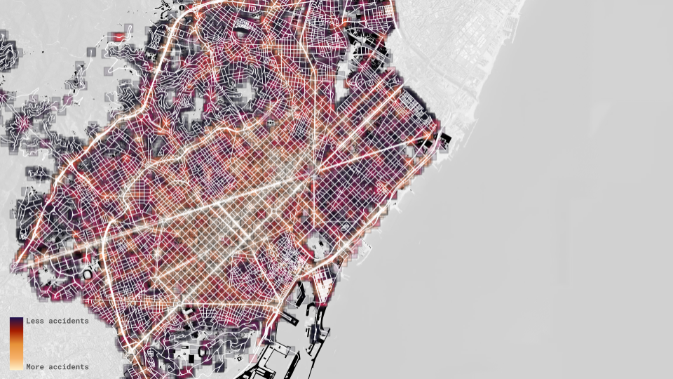
With all pertinent data collected, we create a dataset of 10,000 random samples, each covering 200×200 meters of Barcelona’s streets and their context. These samples are converted into black-and-white 512×512 images using the Grasshopper plugin Squid. Each sample is tagged with the number of accidents that have occurred within the 200×200 meter buffer. These images then become the dataset with which the ML models will be trained.
Models and Training
With an image dataset constructed the models the next step of the pipeline is to train the machine learning models, and visualize their output. For this step multiple models were considered including KNN Regressors and Variational Autoencoders, but in the end due to their simplicity and functionality the following models were selected.
PCA
PCA is a machine learning algorithm which is commonly used to reduce the dimensionality of a given dataset. The way that PCA does this is by combining highly related attributes of a dataset and replacing them by a new attribute that encodes their relation by projecting the data to the axis of highest deviation.
The strength of this algorithm and the reason to use it, is its ability to reduce the amount of data without necessarily losing the abstractions or features that that data encodes, this makes training other models computationally less expensive and avoids redundancy leading to better results.
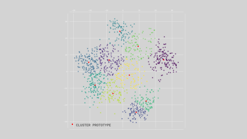
KMeans Clustering
K-MEANS CLUSTERING is an unsupervised ML algorithm used to classify the datapoint in a dataset into a given amount of groups. It performs this task by creating centroids that will act as the prototype or average of a group and iteratively tweaking them by measuring the nearest neighbor distance to maximize the distinction between groups and minimize the deviation within groups.
K-MEANS is powerful and commonly used model that that can help us understand the relation between multiple datapoints by providing a prototype that unites them, but although it is a quite useful algorithm the fact that the amounts of groups to classify the data needs to be predefined means that requires a good amount of fine-tuning.
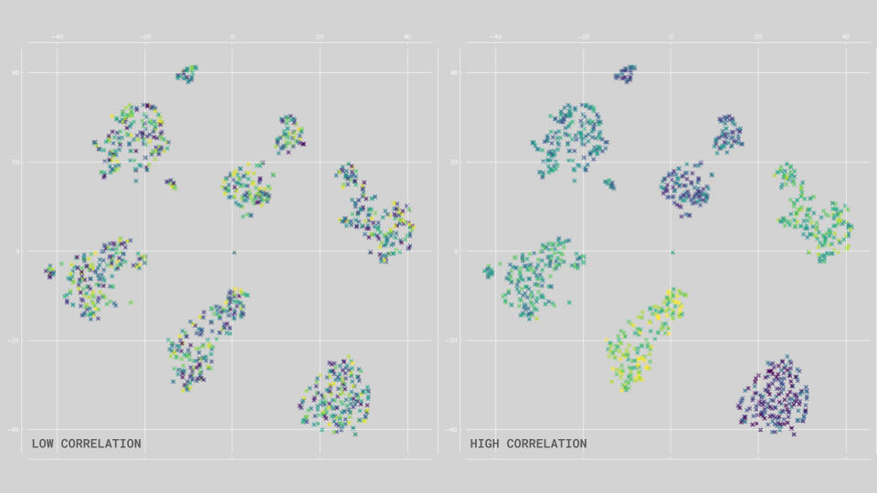
TSNE
TSNE (t-Distributed Stochastic Neighbor Embedding) is an algorithm/technique of dimensionality reduction used for visualizing higher dimensional space. The algorithm project a whole dataset in the 2D plane by keeping similar datapoint -”neighboring datapoints”- close to each other in space.
This technique is useful to better understand how directly related the morphology of the street is to the number of accidents that took place in said street. By plotting the samples and then coloring them based on the amount of accidents and then analyzing the distribution of the color we can understand not only how related accidents and morphology are but also which morphologies are more prone to traffic accidents.
A random color distribution indicates a lower correlation between morphology and accidents whereas a more cohesive distribution indicates a stronger relation and shows which family of street designs are more prone to accidents.
Grasshopper does not natively support machine learning or AI algorithms. To integrate these capabilities, we utilized models from the popular ML Python library SciKit-Learn, accessed through the Grasshopper Hops component. Using the Hops component not only provided access to machine learning models but also made the pipeline fully accessible within Grasshopper. This allowed us to set and edit model parameters and run the models directly from the software. Additionally, the component facilitated the visualization of the model outputs by providing coordinates, labels, and image file paths, enabling us to effectively visualize the training results.
The use of the models required some experimenting to get the best results, but after a bit of fine-tuning the best performing parameters were:
- PCA: n_components=300
- KMeans: n_clusters=15
- TSNE: learning_rate: 250, perplexity: 35, angle: 0.2
Analysis of Outputs
The output obtained from Hops after running the models shows not so well defined clusters that bleed one into each other, but still some main groups of different sizes can be made out from the set of points.
As explained previously the samples positioned in accordance with the TSNE result are then colored based on the amount of accidents each sample had, and based on the distribution of the color we can determined how related the morphology is with the quantity of accidents.
In this case the color is not fully cohesive but rather there is a good amount of randomness to it’s distribution, nevertheless it is possible to still get a sense of a pattern to the distribution, the small cluster in the bottom-left being the one with more accidents. This distribution shows that even though morphology is related with the traffic accidents it is a weak link or at least not a fully direct relation.
In addition to using the PCA & KMeans in combination with the TSNE to evaluate the relation between the morphology and the quantity of accidents of the street networks, the KMeans provides us with prototypes or centroids that can be turn back into images and to have a perspective on what the model is considering as the average of each cluster of samples.
From plotting the respective prototypes for the 15 KMean clusters it is evident that the algorithm found that straight single streets and normal crossings are the best averages for grouping the samples. Although in part this can be attributed to the large amount of barcelona streets that are gridlike (e.g. Exaimple) in comparison with more convoluted streets networks (e.g. Gotico), it has also to do with the limitations of the model, and it a sign that higher level ML models that can better understand the features in a image, might be required.
Comparing variations of dataset
By using hops to create a pipeline that generates the image dataset from shapefiles, then uses them to train the models and finally outputs the results. It is possible to train, visualize and compare multiple variation of the dataset were different information can be display.
Conclusion
Urban Morphology & Traffic Accidents
The PCA and KMean models with the visualization of their outputs via TSNE, permitted to understand how strong the relation between the different morphologies of street and the amount of traffic accident was. The ability of the train models to
The analysis of the output of this models led to the conclusion that even though there is a relation between the accident and the geometry of the streets is not strong one, which means that to get a better understanding and to possibly be able to predict how prone a street is to being the backdrop to a traffic accident, only having the spatiality of the street isn’t enough. Even when adding more geographical information like the position of traffic lights and signage just focusing in the geography is not enough to completely understand what makes an accident happen in a certain street.
Software & Tools
The use of Hops was key to allowing access to the ML models that Python Libraries can offer, and in addition became essential for creating a pipeline that can be abstracted for the training of models on other Shapefile > Image datasets, or even extended to make use the more complex ML models like Autoencoder, GANs and other Neural Networks.
