Roof albedo, the measure of a roof’s reflectivity, significantly impacts urban heat islands, energy consumption, and overall building efficiency. This study aims to analyze how different roof features and materials affect roof albedo in Copenhagen using machine learning techniques.
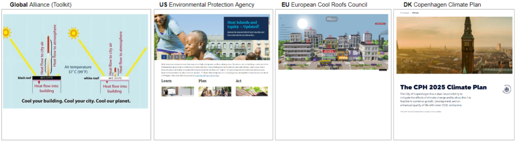
Extreme heat events are rising globally and projected to increase in frequency and intensity, posing a major threat to human health. Cool Roofs are one of the simplest and most cost-effective strategy that cities can use to reduce the urban heat island effect. These references, some significant reports, should provide a robust foundation for understanding the implementation and benefits of cool roofs in Copenhagen and similar urban environments at a Global Level.
There is also another interesting initiative we have investigated, Google Research’s Cool Roofs Lab that allows urban planners to understand the roof reflectivity at the city and sub city level, and combine it with socio economic data such as median household income along with temperature data, to determine areas within their cities that would benefit most from cool roofs.
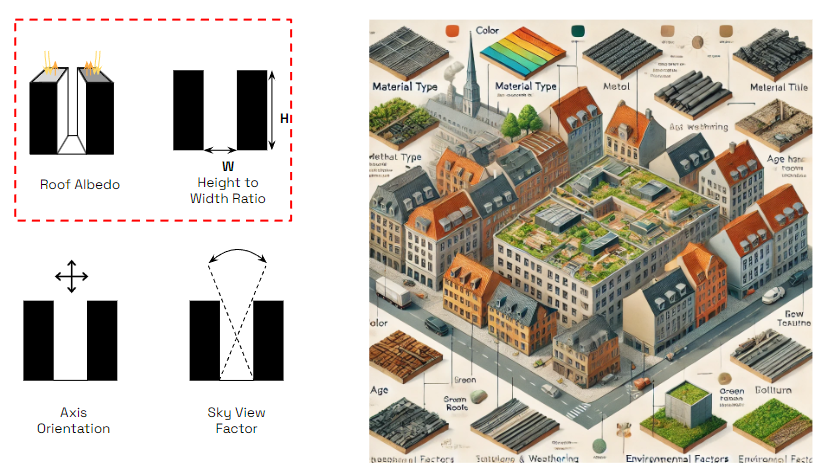
Urban Heat Island (UHI) effect is influenced by several phenomena: Impervious surfaces (buildings, roads, pavements, rooftops), lack of vegetation (reduced shading, lower evapotranspiration), human activities (transportation, industrial activities, energy consumption), building materials (thermal properties, color and reflectivity), urban geometry (street canyons, sky view factor), pollution and greenhouse gases (air quality, greenhouse gas emissions). So among thee features the rooftops were were particularly interesting for our case. Here you find some diagrams illustrating the factors that affect roof albedo in an urban context like Copenhagen. This visual representation includes labeled sections for various influencing factors such as material type, color, texture, age and weathering, roof slope and orientation, environmental factors, and the presence of green roofs.
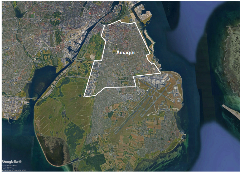
LOCATION: COPENHAGEN, DENMARK
PROJECT AIM
The approach we followed in order to navigate through the roof material investigation and its direct effect on environmental parameters is illustrated in the diagram above. The GOAL is to create a product that allows the user to choose a roof id – from open street maps and predict its roof albedo. Roof albedo refers to the amount of solar radiation reflected by the roof surface. The composition of the dataset is such to allow the training of the modell, that will be presented soon included both geometrical data – roof height and shape for exemple, roof material properties, and building typology information. The machine learning methods are also going to be presented in detail.

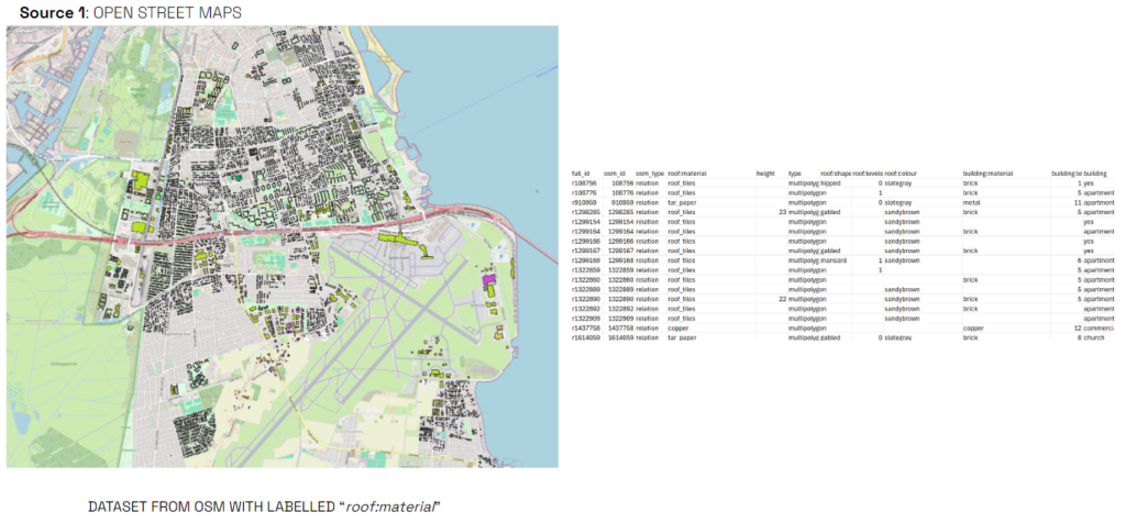
Explaining the dataset composition more in detail, we are presenting 4 data sources: First OSM – where we mark with black color which buildings have rood:material label. We could extract 5 different materials – most represented in the available pool of data, building height, levels, roof typology, shape and colour. https://www.nearmap.com/au/en/products/ai-aerial-maps?utm_source=google&utm_medium=organic. Due to the general incompleteness of the roof color and roof shape labels through osm we also ran a random forest classifier with an 90% and 80% accuracy respectively to predict the missing roof color and roof shape from our dataset based on the other features in our dataset.
DATASET COMPOSITION

A big part of our dataset was data derived from landsat satellite imagery specifically, Land Surface Temperature which represents the temperature of the Earth’s surface as measured from space. It provides information about the thermal characteristics of the land surface. NDVI is a numerical indicator that uses the reflectance of near-infrared and red wavelengths of electromagnetic radiation to assess vegetation health, density, and distribution. It ranges typically from -1 to +1, where higher values indicate healthier vegetation and Fractional Vegetation measures the proportion or fraction of a pixel that is covered by vegetation, providing insights into land cover types and changes in vegetation density. These were gotten by compositing specific bands data from the satelite.
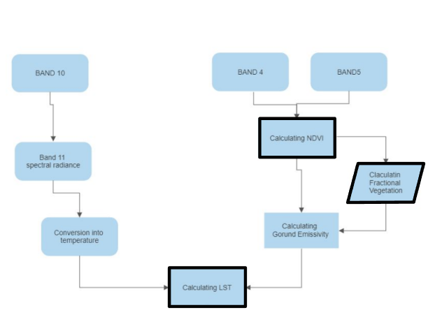
IMAGE PROCESSING (30M RESOLUTION)
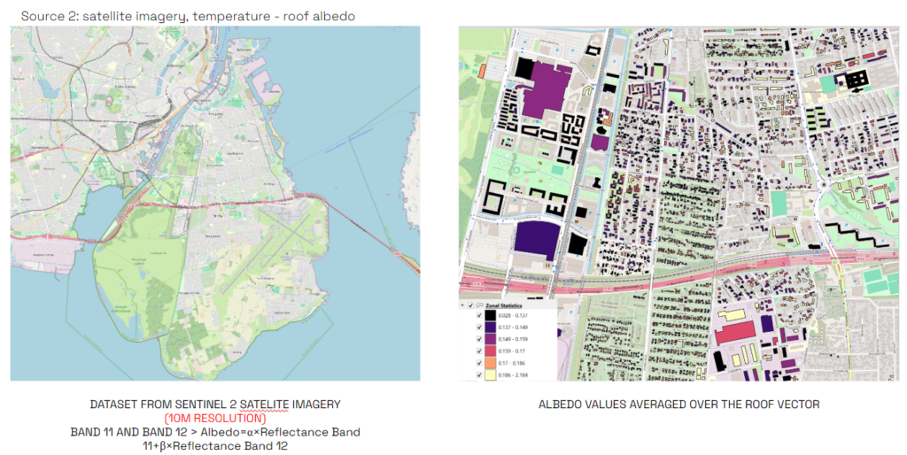
We also calculated the roof albedo from sentinel 2 imagery also by compositing several image bands. And then average the values above a roof vector to get the specific value, which was also done to the previous landsat satellite images.
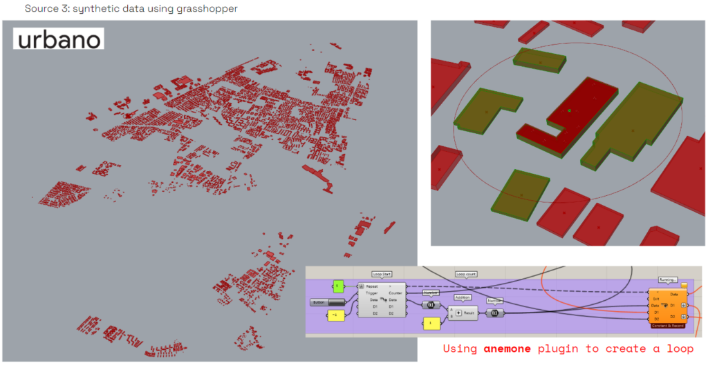
By using urbano plugin , we imported the OSM data & geometry , into grasshopper , in order to do the UTCI calculation & to get geometry data also. as the model is very heavy , we used a loop to divide each building with the closest buildings around it , to be part of the analysis . & to get more accurate UTCI values .
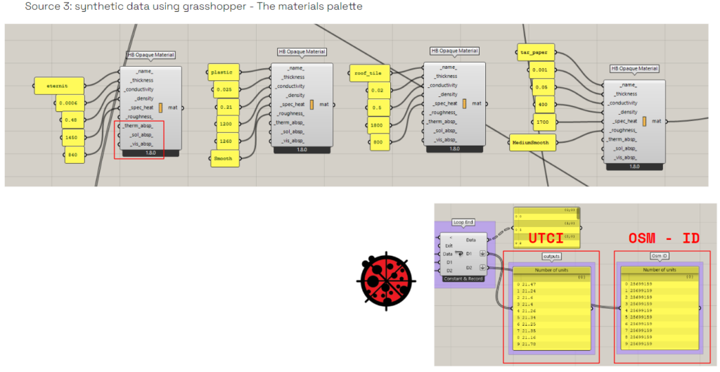
Not all materials are available in the ladybug presets material , so we create the required materials by using the physical properties for our materials .
And then after doing analysis by using ladybug tool , we ended up with UTCI values that are attached with Each OSM ID number for each building .
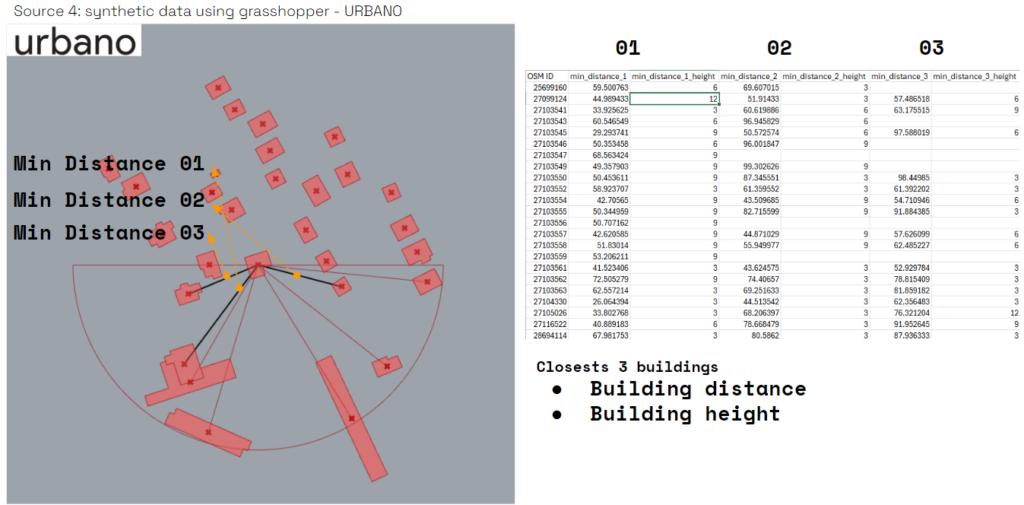
by using same urbano geometry
We used this method to encode the context around each building ,
In the case we took the 3 closest building in the south side ,
Complete Dataset
This is the resulting complete dataset with all of the features
Dataset Analysis
We analysed the spread of albedo values within the dataset and the frequency, we also measured the frequency of materials within our dataset which we tried to make as balanced as possible, and finally measured the spread of albedo values based on materials. So plastic has the highest albedo value meaning that it reflects more solar radiation and absorbs less of it, whereas tarpaper generally has a lower albedo value when compared to the rest of the value, meaning that it absorbs more solar than the others.

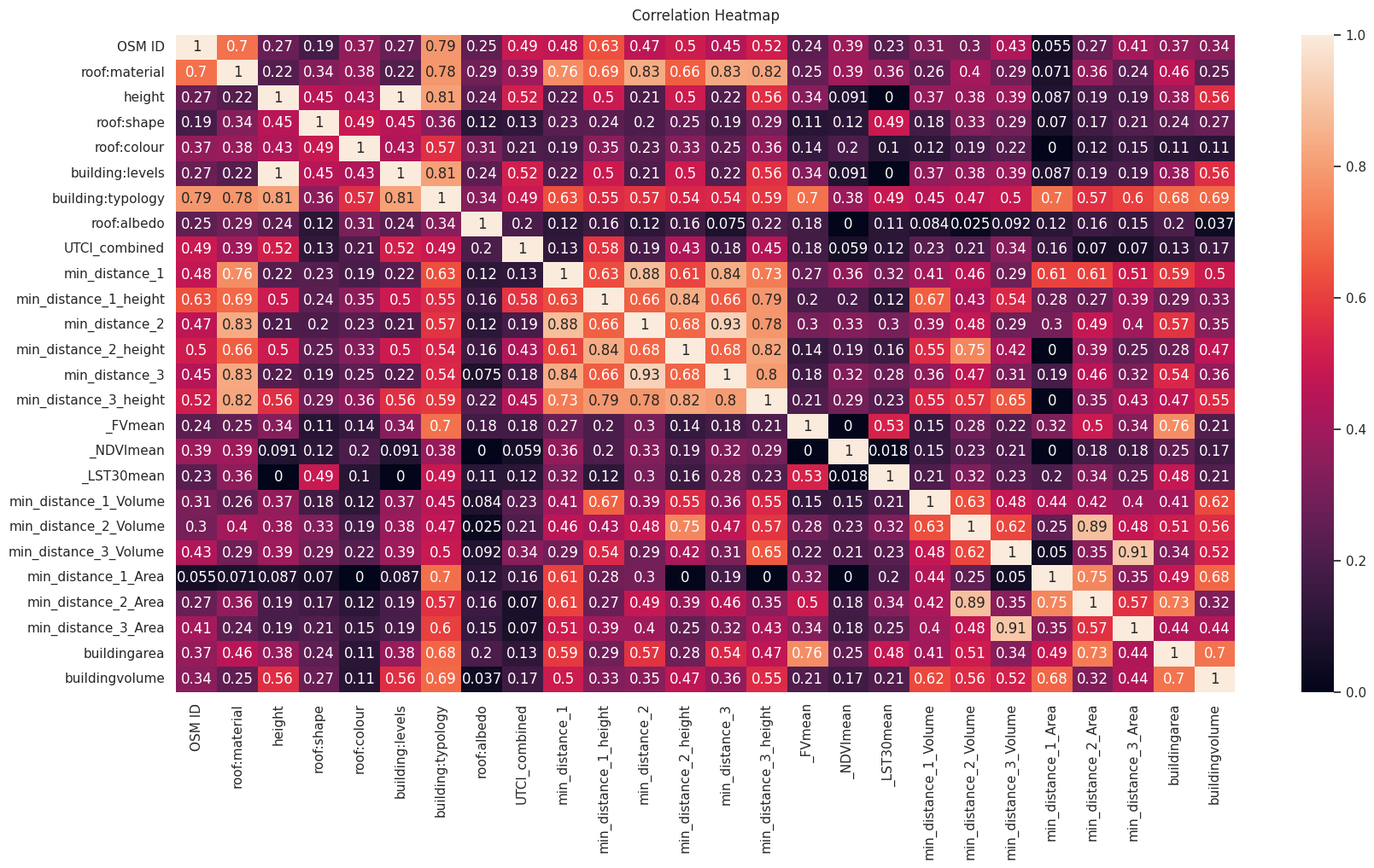
Correlation Matrix
From the complete dataset, we analysed the correlation matrix and kept values that were correlated with the roof albedo, even though NDVI had 0 correlation with roof albedo we found that removing that during training reduced the model performance suggesting that it may not have a linear correlation with the albedo but may be correlated with other values that influence the albedo. We also extracted more information of the context like the area of the roof being analysed and the volume of both the building and the closest 3 buildings, we also observed a reduction in performance when those features were introduced. So th feature selection was an iterative approach all through training.
PCA Analysis
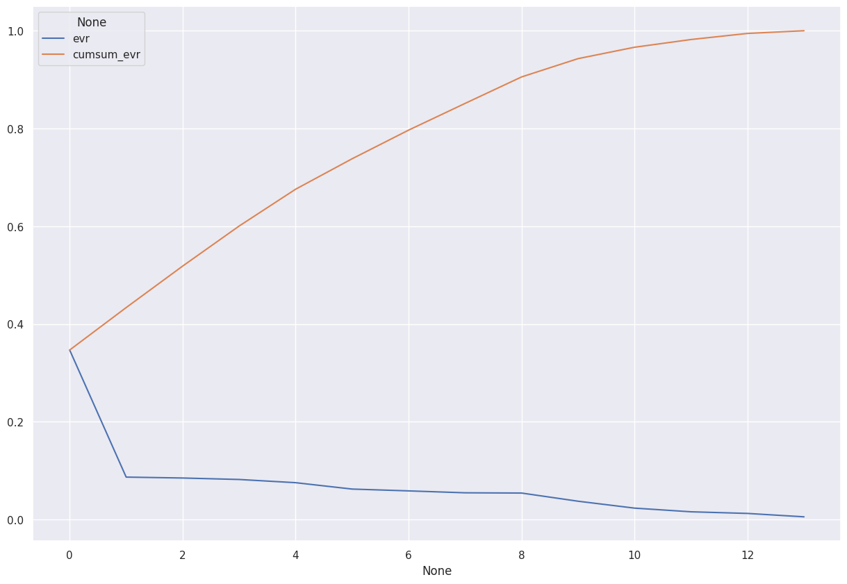
We ran a pca analysis with 13 features selected and found that we didn’t not need to use a pca because the graph converges at 1 at slightly above 12 on the x axis which is similar to the number of features we had, hence no dimensionality reduction was necessary.
Linear Regression
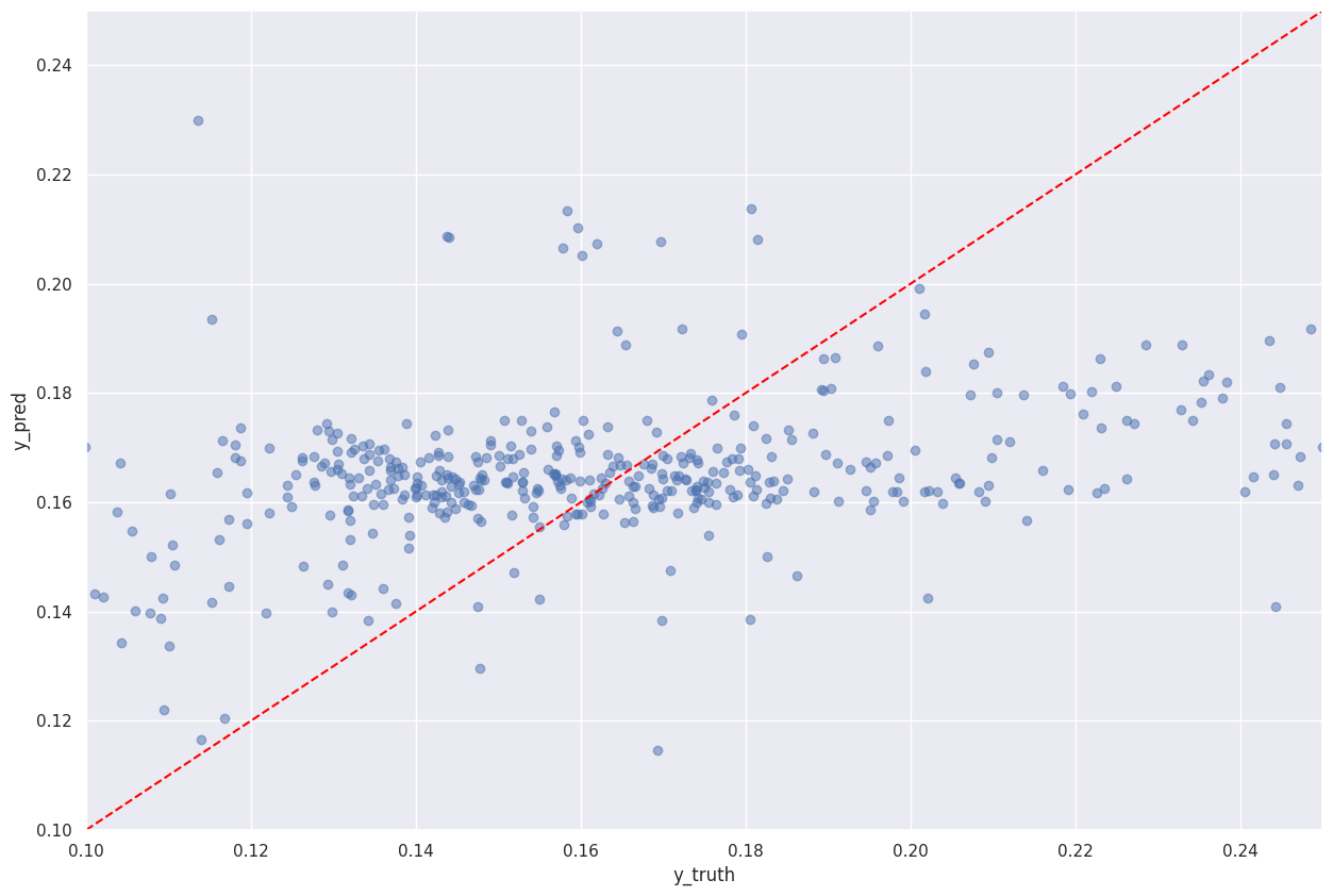
The first model we tested with our dataset was a shallow regression model, with a performance of 7% and a bad looking plot against the diagonal line, we concluded that this was not the right model and there were relationships within the features that were non linear.
Model Performance: 7%
XGBoost
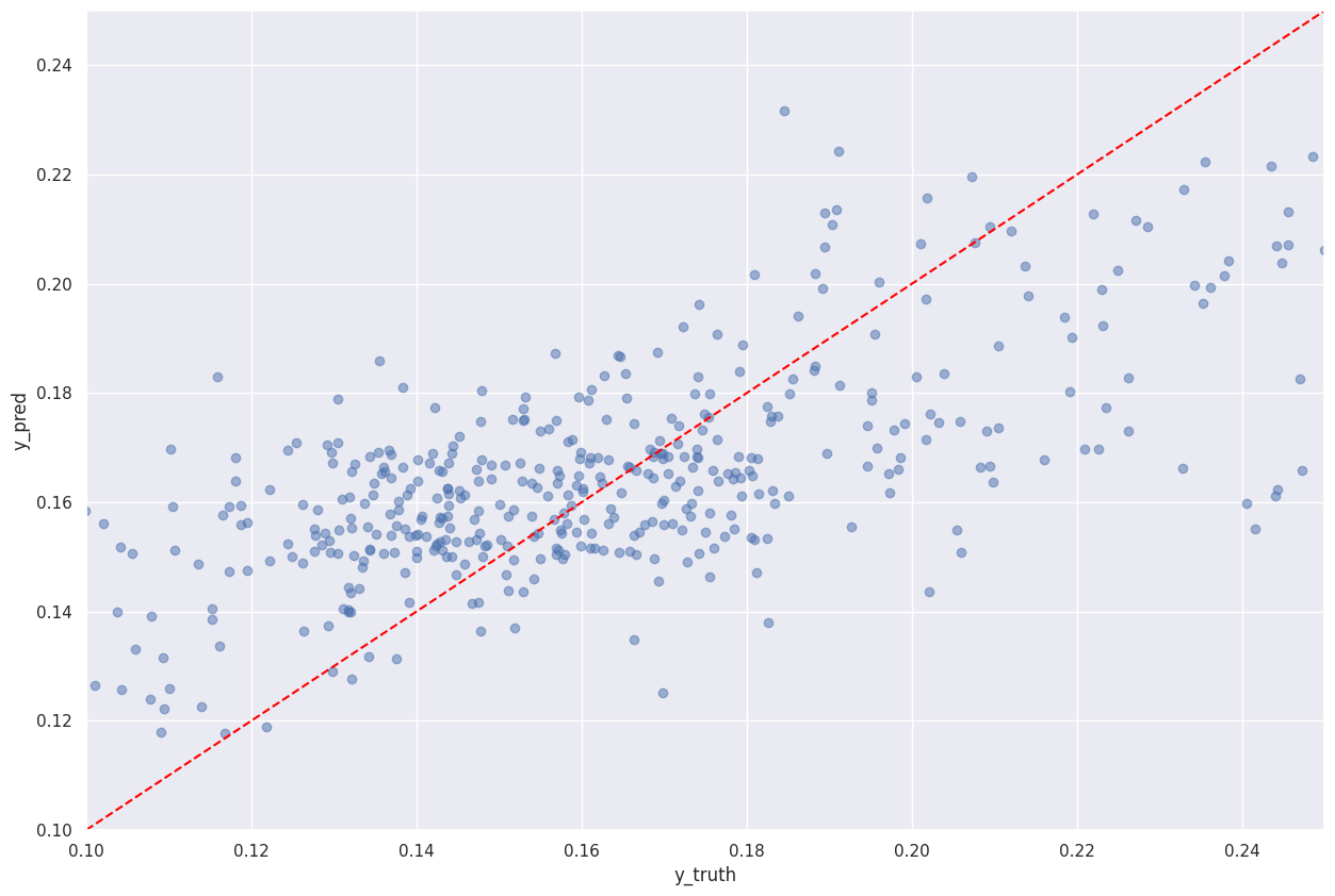
We started to get a lot more success running an XGBoost model with a learning rate of 0.01, maximum depth of 6 and the number of estimators of 300 as the best parameters we found.The performance gave a maximum score of 28.5% with a slightly better graph when compared with the previous.
Model Performance: 28.5%
ANN Regression
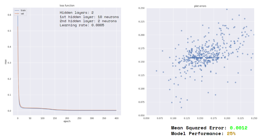
An artificial neural network gave a us a slightly lower model performance when compared to the previous XGboost with a drop of about 3% in performance to 25%. We used 2 hidden layers, the 1st with 10neurons and the 2nd with 2, with a learning rate of 0.0005. When plotting the errors, you can observe that there is quite a few.
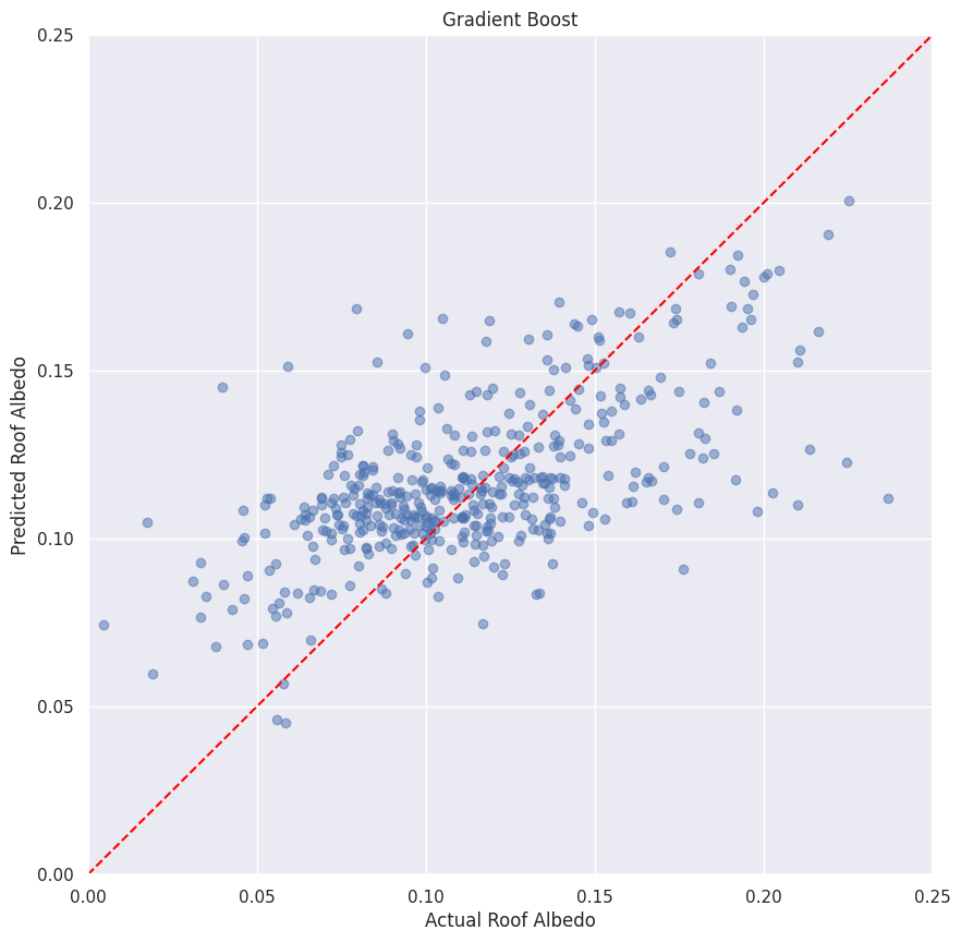
Gradient Boost
We started to get more significant success using a gradient boost model with a performance of 37%
Model Performance: 37%
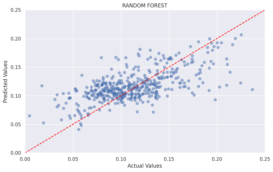
Random Forest
And finally the most successful model we found was a Random Forest model taking us up to 40% with a learning rate of 0.01, and a max depth of 5. After several iterations of adding more features or removal we found that 40% was the best we could achieve with this model. In conclusion, the random forest model served us better to predict the albedo and a potential room for improvement would be even more feature engineering, to help the model read more connections within the dataset.
Model Performance: 40%
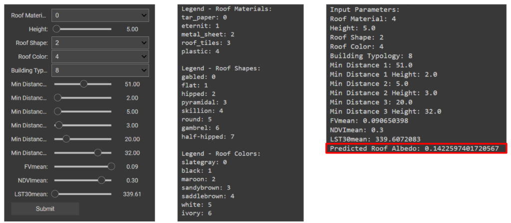
Collab UI
From this we created a public google colab file with our saved out pickle model, label encoders for categorical variables, and the standard scaler, to recreate a UI where the user can input values of their roofs to see the predicted albedo, using ipy widgets. This is a quick proof of concept of how users can interact with a trained ML model without the need to access the training information directly. The input parameters are set within the bounds of the dataframe for better predictions and the legends of the label encoder is displayed for better interpretation of the results.
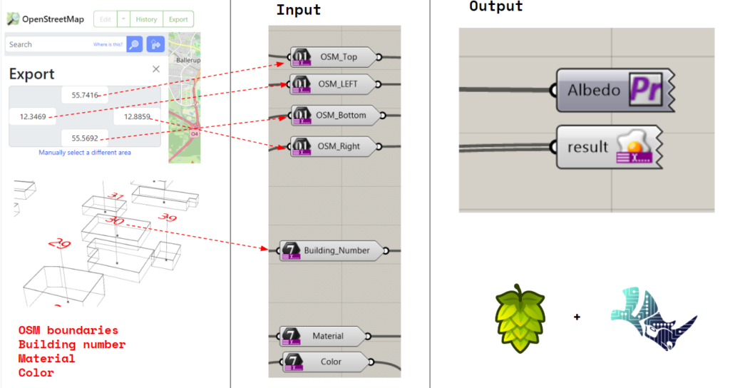
Hops
Also , we aimed to deploy the tool in a web based app .
To give the opportunity to anyone to access the tool .
So , We used hops & rhino compute .
Defining our inputs and outputs ,
As hops will help us to use rhino compute in the cloud ,
We hope that we have more time in order to make this app working .
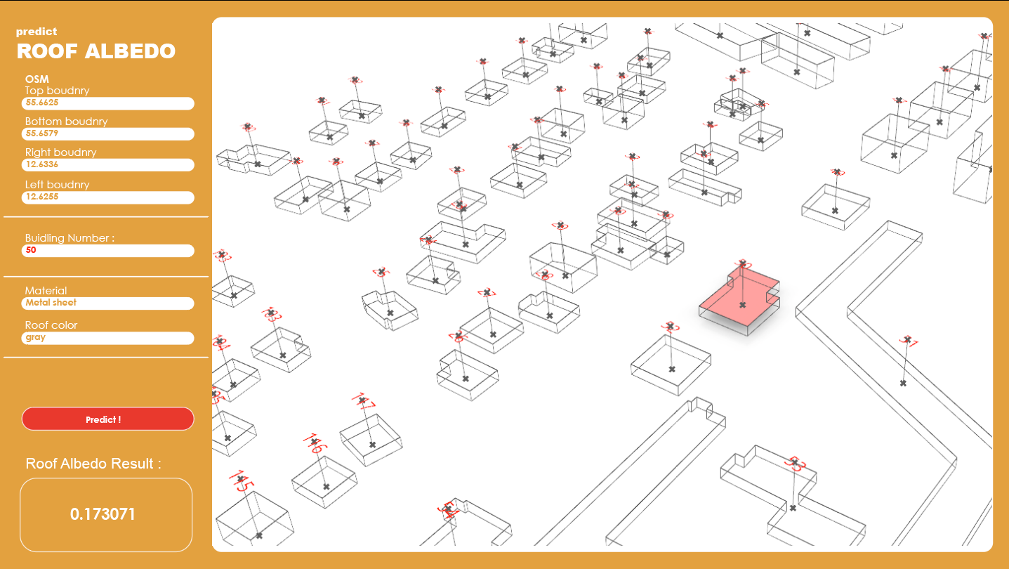
But we are showing this graphical interface to explain how the user will interact with our app .
In order to predict the Albedo in a real world context .
the user will input OSM boundaries , and building number to select one building & different materials & colors options .
And then the albedo result will be predicted by using our AI model inside rhino compute .