NYC Taxi Trip Duration Predictive Modeling

The objective of this exercise is to build a machine learning model that will predict taxicab trip durations based on 2016 NYC Yellow Cab trip record data.

Data Fields

• id – a unique identifier for each trip
• vendor_id – a code indicating the provider associated with the trip record
• pickup_datetime – date and time when the meter was engaged
• dropoff_datetime – date and time when the meter was disengaged
• passenger_count – the number of passengers in the vehicle (driver entered value)
• pickup_longitude – the longitude where the meter was engaged
• pickup_latitude – the latitude where the meter was engaged
• dropoff_longitude – the longitude where the meter was disengaged
• dropoff_latitude – the latitude where the meter was disengaged
• store_and_fwd_flag – This flag indicates whether the trip record was held in vehicle memory before sending to the vendor because the vehicle did not have a connection to the server – Y=store and forward; N=not a store and forward trip
• trip_duration – duration of the trip in seconds

Based on this, this project will develop a machine learning regression algorithm capable of predicting the duration of a trip based on the variables provided by the application user (passenger) and the driver.

Process

1. Data Preparation & Feature Engineering: A preview of the data will be done, in order to identify and treat inconsistent and missing data, in addition to creating extra features based on the initial features.
2. Correlation: The correlation between the data will be analyzed in order to avoid possible multicollinearity problems.
3. Data Visualizations & Analysis : Visualizations will be performed in order to find relevant insights for the development of the algorithm.
4. Filtering the Outliers
5. Running Prediction Model: It is the stage where the machine learning model will be created and evaluated, where the hyperparameters of the model will be tuned in order to improve the model result, and the feature importance analysis of the final model will be carried out.

1. Data Preparation & Feature Engineering

Clean and transform the data into a usable format for analysis for examples changing the data type of the columns ‘pickup_datetime‘ and ‘dropoff_datetime‘ from object to datetime64[ns] . Creating columns like ‘Trips Distance’, ‘Pickup_(day, hour, minutes and seconds)’ and ‘Dropoff_(day, hour, minutes and seconds)’ from the given data in order to analyse it.

2. Correlation

3. Data Visualizations & Analysis

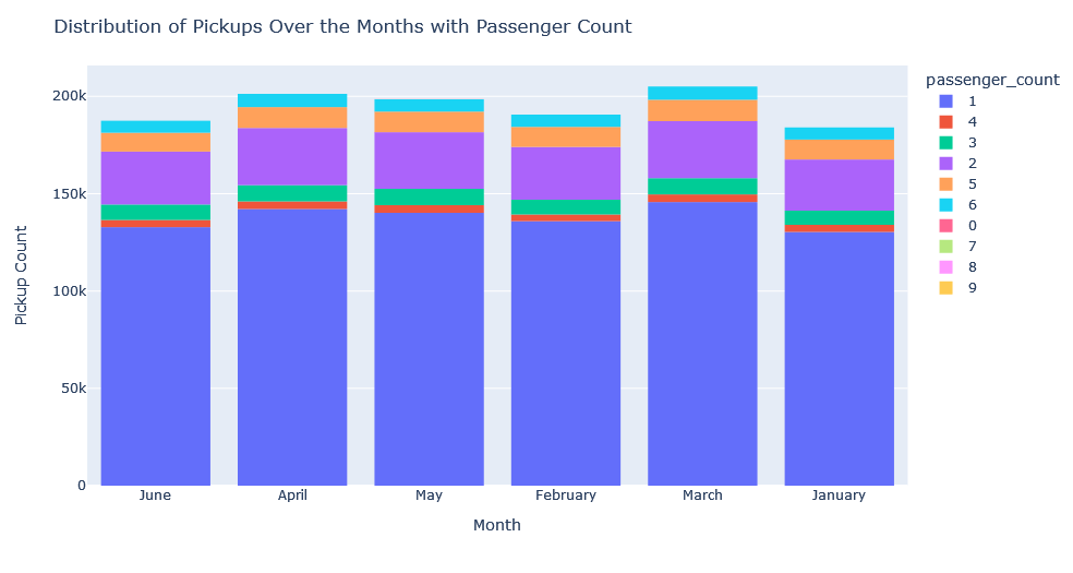
From the graph of the months, it can be seen that all months have values close to the amount of data, with the lowest value in January and the highest in March.

From the day week pickup graph, it is possible to observe that the days of the week do not have a relevant difference in the amount of data. Monday and Sunday are the days with the fewest trips and Saturday and Friday are the days with the most trips.

4. Filtering the Outliers

‘passenger_count’ : New York City Taxi Passenger Limit says:

• A maximum of 4 passengers can ride in traditional cabs.
• A child under 7 is allowed to sit on a passenger’s lap in the rear seat in addition to the passenger limit.

So, in total we can assume that maximum 5 passenger can board the new york taxi i.e. 4 adult + 1 minor The variable has a minimum value of 0 passengers, which does not make sense in the context of this business case. These observations are most likely errors and will need to removed from the dataset.\

‘pickup’ and ‘dropoff’_Coordinates: Based on different coordinate estimates of New York City, the latitude and longitude ranges are as follows:

• Latitude is between 40.7128 and 40.748817
• Longitude is between – 74.0059 and – 73.968285

The statisical summary of pick-up and drop-off coordinates show max and min observations that fall outside of the NYC city coordinate range. These data points can be excluded as this analysis is limited to New York City.

‘trip_duration’: There are unusual observations present in our target variable, trip_duration. A maximum trip_duration of 3526282.00 sec (~ 980 hours) is not a realistic trip time – a clear indication that outliers are present in the data. A systematic way to remove these outliers is to exclude all data points that are a specified number of standard deviations away from the mean. In this case, drop trips with duration less than 1 minute or greater than 2 hours

‘trip_distance’: To drop trips with distance less than .5km or greater than 50km (maximum distance that can be travelled) in corresponding with removal of other outliers

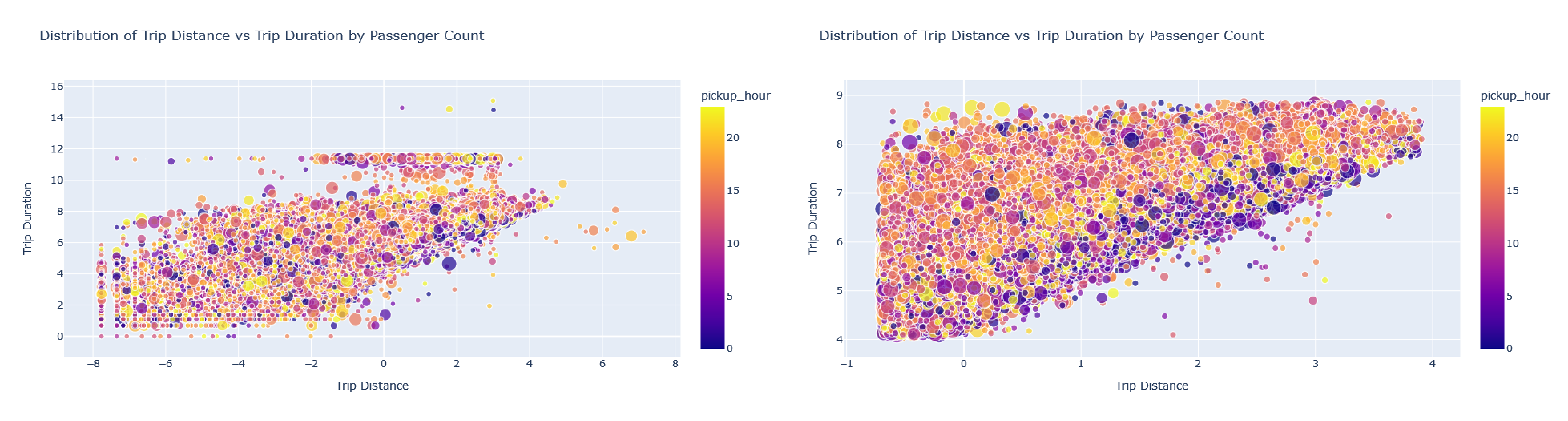
Scatterplot: Distribution of ‘trip_distance’ vs ‘ trip_duration’ by ‘passenger-count’ with the outliers (left) and without outliers(right)

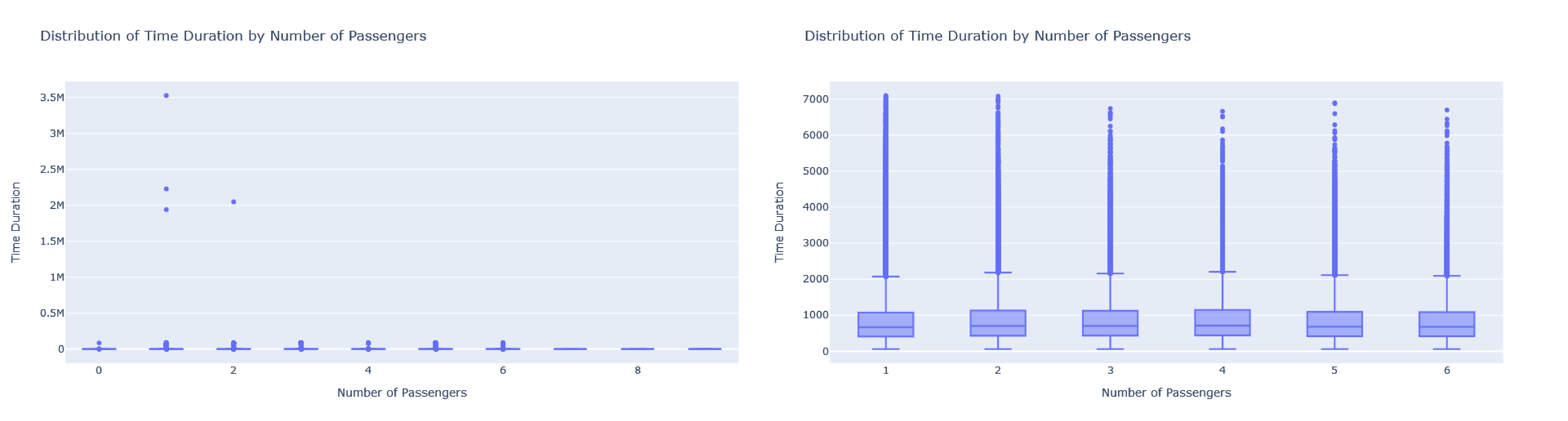
Scatterplot: Distribution of ‘trip_duration’ vs ‘ passenger_count’ with the outliers (left) and without outliers(right)

5. Running Prediction Model: Random Forest Regressor

Before applying the regression model, the normalization of non-categorical data will be applied, aiming to increase the performance of the model and prevent the algorithm from becoming biased towards variables with a higher order of magnitude.

To run the prediction on the trained model foloowing are the chosen columns ‘passenger_count’ , ‘pickup_longitude’, ‘pickup_latitude’, ‘dropoff_longitude’, ‘ dropoff_latitude’, ‘pickup_hour’, ‘ dropoff_hour’, ‘pickup_min’, ‘dropoff_min’ and ‘trip_distance’. In this case, all data for model training is used to increase the performance of the generated algorithm, thus increasing the results with the final test data. Random Forest Regressor was applied as a prediction model as it gave better results than other regression models.

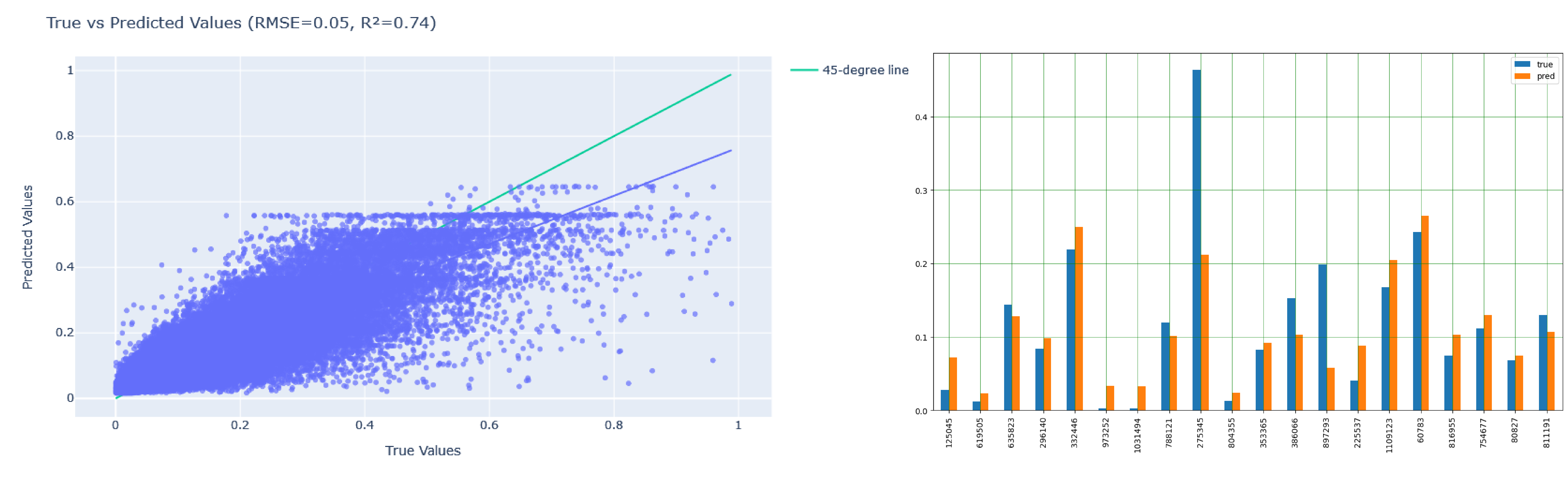
The result obtained from the algorithm was close to the expected result in some cases with R² Score = 0.74 and Root Mean Square Error (RMSE) = 0.05, and it is expected that when applied to the test data similar results will be obtained.