Find the perfect seat in a stadium!
Problem Statement
How many times have you been to a stadium, sports complex, concert or related events where your seat look much less appealing than in the sales chart?

This raises a very important question, what are the metrics used to define the quality of a seat in a stadium, concert hall..etc.
Classic Visibility Metrics
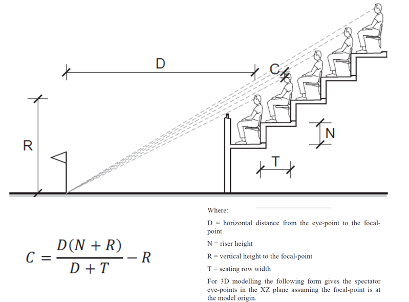
C-Value
the vertical dimension C (the c-value) between the eye-point of one spectator and the sightline of the spectator behind, originated from 1838.
In this 2D system, views are oriented perpendicular to the spectator’s shoulders and always positioned above the heads of spectators in front.
Simulating Human Visual Experience in Stadiums Roland Hudson1 and Michael Westlake2
In this 2D system, views are oriented perpendicular to the spectator’s shoulders and always positioned above the heads of spectators in front.
A major limitation to this metric is its two dimensional nature, usually fails to capture third dimensional aspects of the analyzed geometry.
A-Value
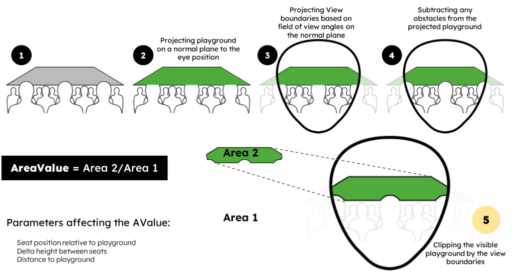
A novel approach to measure seat quality is the A-Value or what so called “Area Value” in this measure:
- A line connecting spectator eye position and a point of interest is drawn.
- A Plane perpendicular to this line of sight is constructed at any position except the position of spectator’s eye.
- Set of lines connecting spectator eye position and playground/show boundary area are drawn cutting the perpendicular plane at specific point so that the area of interest can be projected onto this plane
- Using similar approach view boundary is also projected on the perpendicular plane allowing us to clip the projected area on interest that lies within.
- Again projecting any possible obstacle onto the perpendicular frame.
- Finally calculating the visible projected area of interest percentage to the area of the projected view boundaries
Project Objective
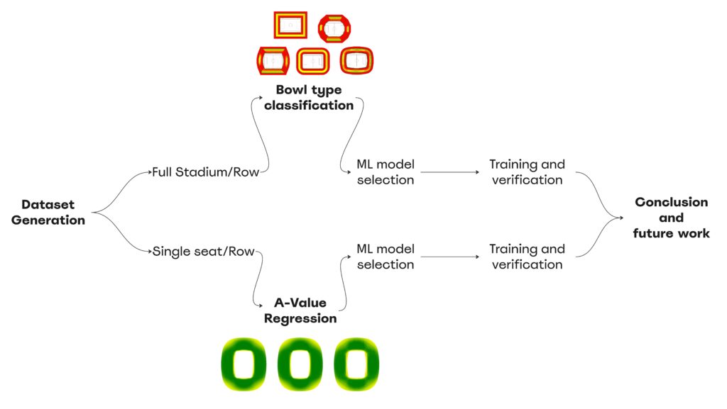
Develop a trained machine learning model that has the ability to calculate and predict the A-Value of each seat in a stadium.
This can be used by designer in the design phase, Marketing agencies for setting seat price and also stadium users to check their seat playground visibility quality before buying the ticket.
Another objective is to try classifying stadium bowl types based on its seats quality.
Project workflow
Dataset Preparation
Defining dataset parameters to encode
Studying the nature of stadiums we can say that there are Three types of parameters used in our dataset preparation:
- Parameters to generate bowl variations to generate good distribution of eye positions.
- Parameters to Encode for the machine learning, these are the trickiest parameters to capture.
- Quality measures for each seat physically calculated in grasshopper ( C-Value, A-Value ).
The first type includes ” Row width, initial C-Value, bowl offset distance from playground, Bowl length radius, Bowl width radius and Bowl corner fillet”
The second type needed some validation to ensure that the encoded features are the ones influencing the change in seat quality.

Generation

Using toros plugin + native grasshopper components we generated different stadium typologies to ensure a good distribution of eye positions
Using bowl related parameters as:
- Row width
- C Value
- Offset distance from playground
- Width radius
- Length radius
- Corner Fillet
Dataset size: 1000 stadiums, 1747200 eye positions

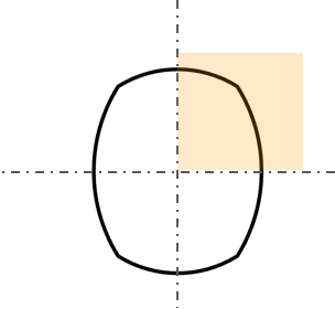
Hence Football Stadiums are usually symmetrical so we decided to present each stadium with only one quarter.
Data Visualization
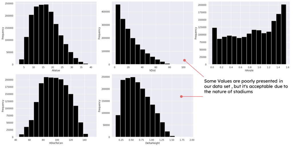
After generating the dataset it was crucial to plot some graphs to ensure good distribution and good correlations within our dataset.
Correlations and outliers check
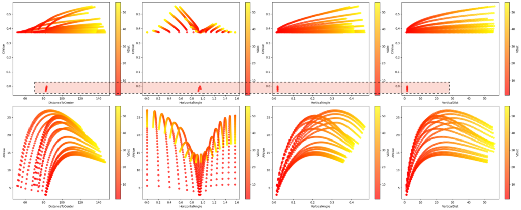
The inconsistent in C-Values are clear
The inconsistent in C-Values are clear
At the beginning we were aiming to train on both A-Value and C-Value, but we encountered some inconsistencies resulting from C-Value usually caused by corners and front seats and normal directions , despite trying to eliminate these inconsistencies they remained as C-Value measure has a lot of exceptions in the way it is calculated, so at this point we predicted that C-Value will be problematic in the training process, however we decided to keep it for now.
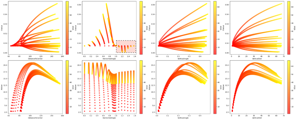
For A-Value, the visualizations showed logical correlations based on the nature of stadiums.
the visualizations showed logical correlations based on the nature of stadiums.
the visualizations showed logical correlations based on the nature of stadiums.
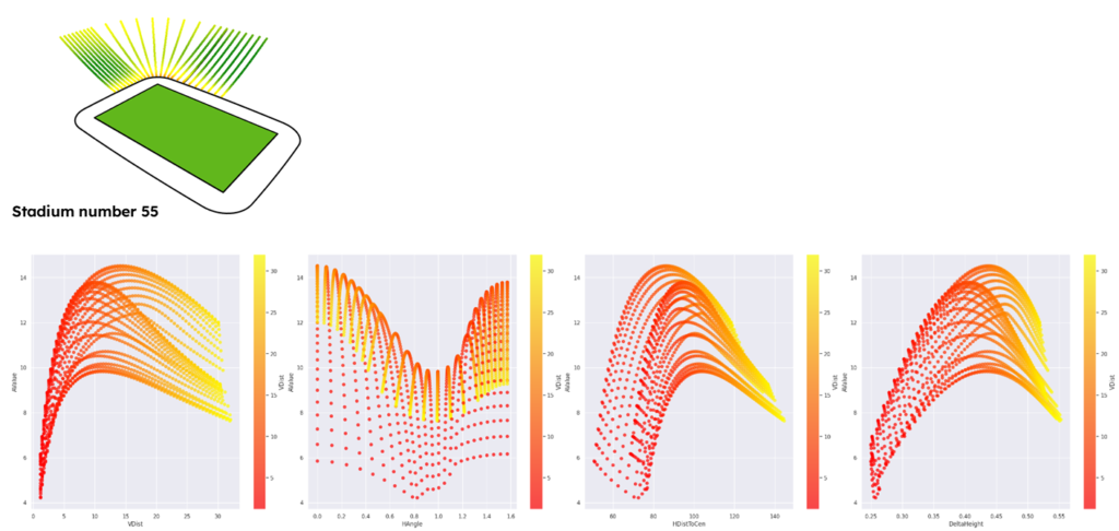
the visualizations showed logical correlations based on the nature of stadiums.
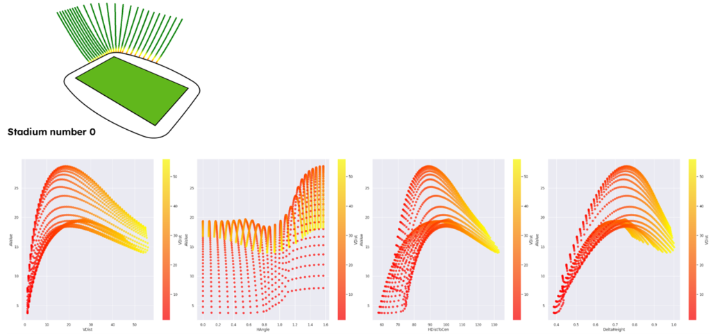
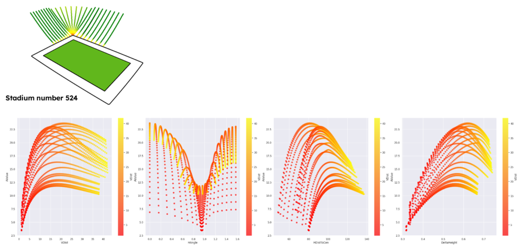
Data distribution check
Single seat/row
ML model selection
First of all our objective is to calculate a certain value so it’s a regression problem.
Going from shallow model to deep ones till we achieve acceptable results.

Model Training and verification
Some Failures!
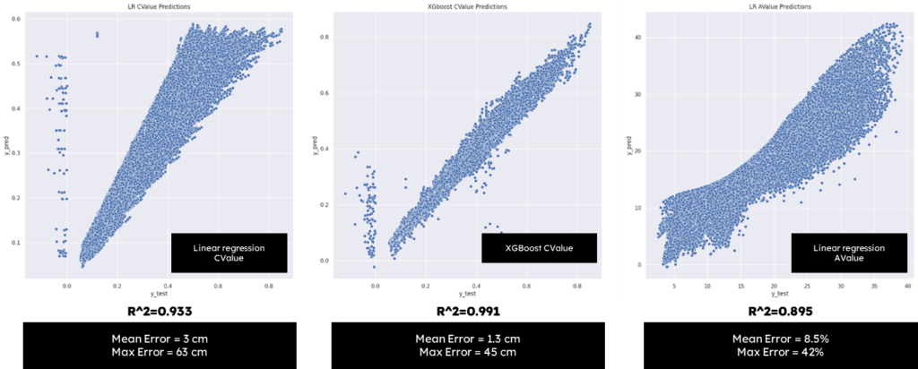
as predicted C-Value prediction showed very poor results in linear regression and XGBoost ML models with lots of outliers, here we decided to drop C-Value calculation part.
Also first trial with linear regression model to predict A-Value showed poor results.
A-Value XGBoost
Using XGBoost from Sci-kit learn we manage to get great results with mean error = 0.425%, a very acceptable score.

The plot on the left show the variation between real A-Value and predicted A-Value using the testing dataset “unseen data by the model”.
The plot on the right is visualizing the error distance between real and predicted value showing only 2000 random points from testing dataset.
A-Value ANN
seeking better results we tried using artificial neural networks from tensor flow, using a shallow network, Trained for 20 epochs with batch size 500.
extraordinary results were achieved with mean error of 0.000023%


The plot on the left show the variation between real A-Value and predicted A-Value using the testing dataset “unseen data by the model”.
The plot on the right is visualizing the error distance between real and predicted value showing only 2000 random points from testing dataset.
Geometrical verification
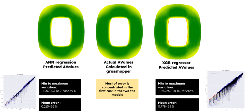
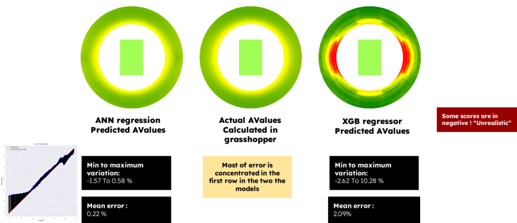
we tested the trained models on data within the training bounds and they both showed good results with ANN always outperforming XGBoost model, then we tested them on unseen out of training bounds stadium the circular typology which was never in the training dataset, XGBoost performed very poorly with unrealistic values but ANN showed remarkable results with very acceptable error margin.
An important observation is that most of error in both models is concentrated in front rows, and this is because front rows specially the first one is calculated with some assumptions rather than physical analysis because there is seats in front of the first row.

Conclusion and future work
Conclusion
Machine learning models were able to predict the A-Value metric for football stadium with good accuracy, however we manage to highlight some facts :
- Neural networks showed higher performance than shallow learning model XGB in all trials and verifications.
- Neural networks showed good ability to generalize on unseen out of training bounds data while XGB badly failed
CValue predictions were very hard to achieve because of the way its calculated has already a lot of exceptions the thing that make it difficult for machine learning models to capture the trends.
Future work
This project was a proof of concept which is for the sake of this exercise was limited to football stadiums with playground of 68 * 105 meters.
A good practice may include variations in playground dimensions to make a more generic model that can perform well on different sports stadiums, however this may require tweaking the stored parameters to include factors that are more sensitive to playground dimensions such as distance to corners.