Abstract
The introductory course of Software I focuses on the computational logic for assamblage and growth processes guided by algorythms. For starting, voxels were created as basic units and then joined to create a basic element geometry. By using Grasshopper and Anemone plug-in, different growth assamblages were established depending on the element’s position and starting growing planes. The knowledges were applied for a final project proposal with personal parameters to generate a final geometry.
Our exploration though the design process helped us understand the technique for growing and assemblage elements guided by different parameters such as growing over Z, avoiding obstacles and growth along an attracting curve.
Components design
For the assamblage exercise, we designed 3 voxel-based components. Each one had 3 different handle positions which generated 9 combinations, having successfull (with no colision) and unsuccessful (with collision) assamblages. The result of the premutation growth was depending on the handle position which leaded to 3 different results in this task, however, more results can be generated if we change the handle position.
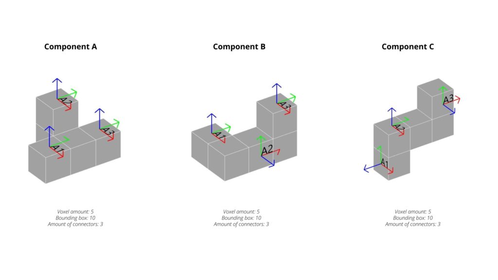
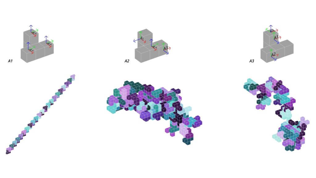
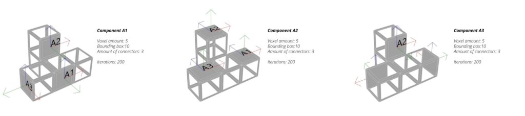
Component A
Component A is based on 5 voxels with 3 handles. The assemblage variation differs depending on the position of the handles. A1 assamblage leads to a linear result because the handles are located towards the same direction. If the handles cover most locations of the element, the result turns more complex. (View on Figure 3, assamblage A1)

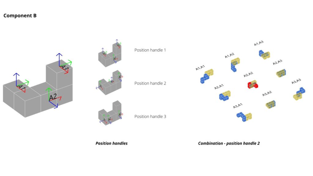
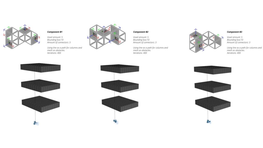
Component B
Component B is also based on 5 voxels with 3 handles. The position of the voxels and handles are the base for the assemblage and growth. At the combination of this component using handles at position 2, there are 8 successfull and 1 unsuccessfull assamblages. The red component at the image below shows the collision between the two components, which is caused by the position handles from A2.
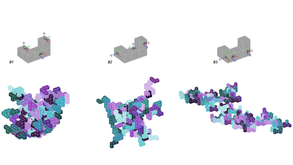
From this component, we concluded that when the handles are located at the same voxel line, the addition result turns more planar. This result is visible at Figure 5, B3 assamblage.
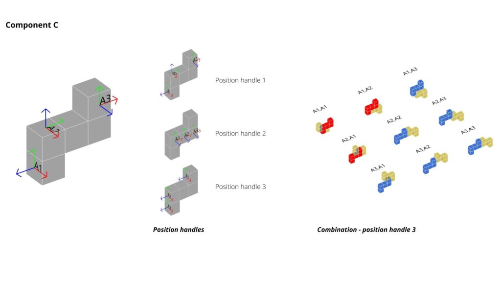
Component C
Component A is based on 5 voxels with 3 handles, just like the others. The difference in this component’s result is due to the handles positions. 3 out of 9 combinations were unsucessfull due to collisions, leaving just 6 successful results.
This handle position on this component were strategically located for experimenting the linear result. The hypothesis from the last teo components was that the more different the location and direction from the handles, more complex the result. In this case, handles on position 3 and 3 were located looking towards the same direction to verify the hypothesis. As you can see on Figure 7, handles on C2 and C3 prove that the result is linear due to the location and direction of the handles.

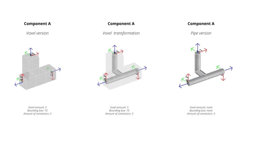
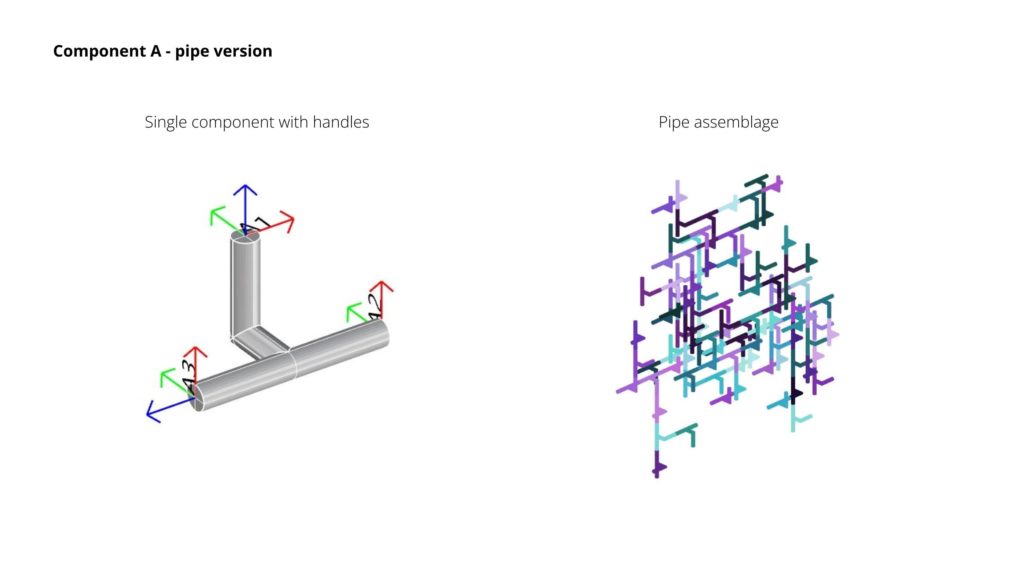
Component A – Internal volume replacement
The voxel was replaced into a piped figure in order to generate a different geometry than just boxes. This strategy was created to demonstrate that the task works for different geometries and the complexity of them can vary as much as the designer wants.
Component A – rotation of handles
Now that we see that the voxel can be replaced to another geometry and used for the same purpose, we made another task by taking the original voxel component and rotating one of the handles, in order to see if the assamblage geometries change due to the rotation. For this, we took handle A1 and rotated it 90° in 4 steps to see and compare the assamblages. In this scenario, we compared them and saw that the result was different, and we noticed that having all handles towards the same rotation lead to a linear result. Rotating the handle at an angle of 90º from the base handles also leads to a linear result (mirrored). (View on Figure 10.)
As an observation, the assemblage result in the 270° rotating angle is planar because the handles are located in the same face direction of the voxels. Locating the faces in any component towards the same direction and rotation will lead to a planar and linear result.

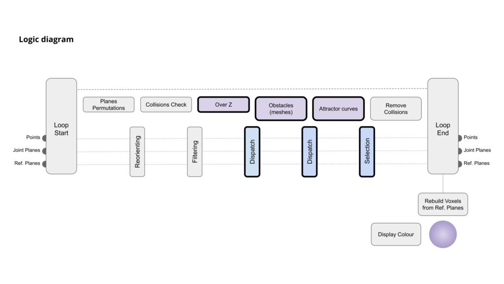
Custom filtering method
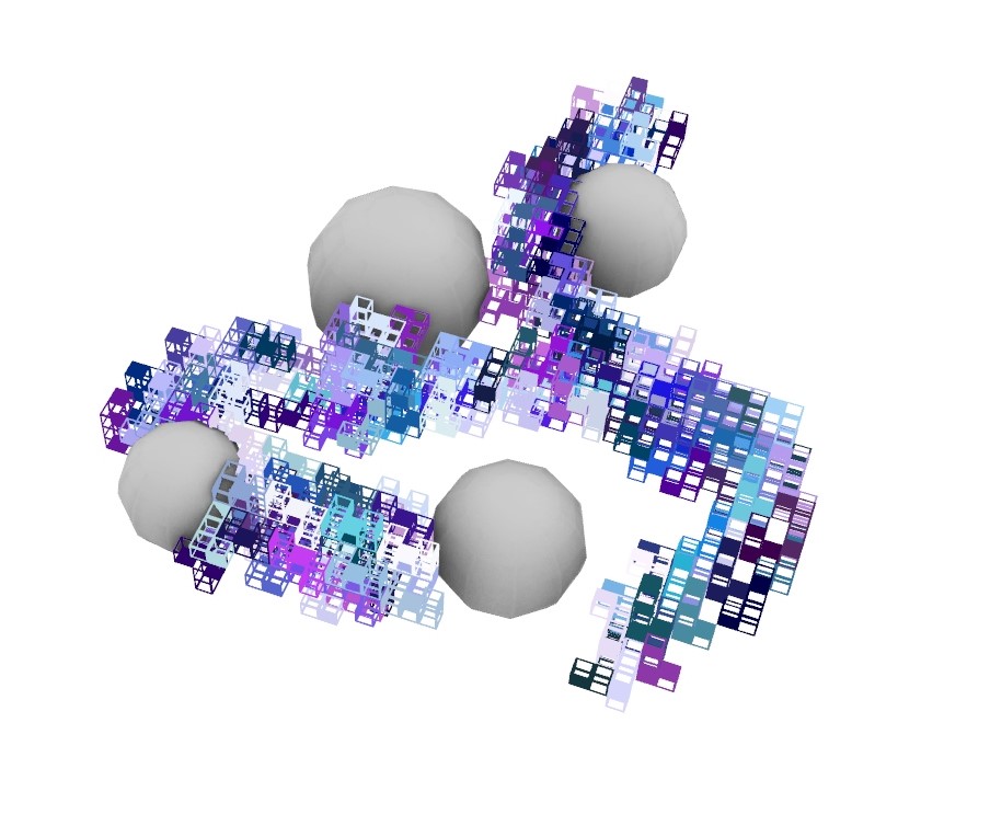
Having the base growth code, we decided to intervene by proposing 3 different types of filtering criteria. The implemented filters were: growing over Z, avoiding obstacles (which are sphere meshes) and following the growth through the attractor curves. On the following diagram, there is a visualization of the addition methods that were implemented in the process for the growth design.
Component A
For the proposal, the design of the voxel component was modified with open faces generating a more light and transparent component. Also, the corners and edges were softened and the handles were located as the first component to have the same growth iteration from the beginning compared to the new growth which includes the filter proposed method. On the image below, the component A is shown with the different set of handles for the experiment.
The way the handles are positioned in the components affect the amount of components following the attractor curve logic. The more dispersed and rotated the handles are, the more coverage of the area. (Component A3 has more coverage than A1 and A2 components).

Component B
The same design was proposed for component B to create a comparison from the first task steps. In this component we positioned a set of 4 handles to see if they affect the amount of components following the attractor curve logic. The more dispersed and rotated the handles are, the more coverage of the area. (Component B3 has more coverage than B1 and B2 components).

Component A3 and B3 comparison
For a better understanding method, the components A and B were compared to see the difference bewteen the assemblages of 3 and 4 handles. Also, depending on the position of them are the successful and unsuccessful components. The final shape with the holes on the voxels is respected and the result differs and depends on the handle postition.

Architectural approach
Using the method implemented with the voxels, we decided to create a column with the growth assemblage following the curve and avoiding obstacles which are the dark grey boxes seen on the image below. The growth is different depending on the handle position but the result can be used for the same structural / architectural purpose.
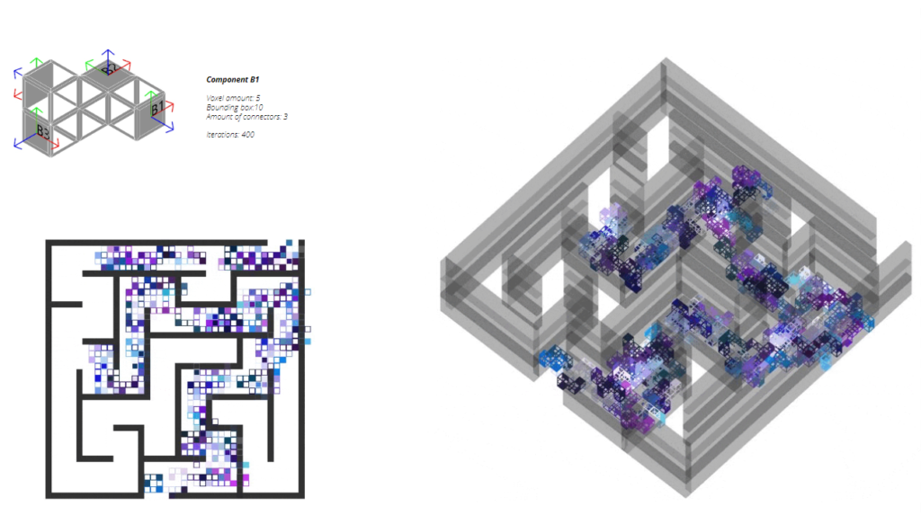
Maze game
The final approach for the project was to create a maze game that follows the same logic: growing from a start point to an end point avoiding obstacles (maze wall). We used component B1 for this experiment and the result is shown on the image below.