
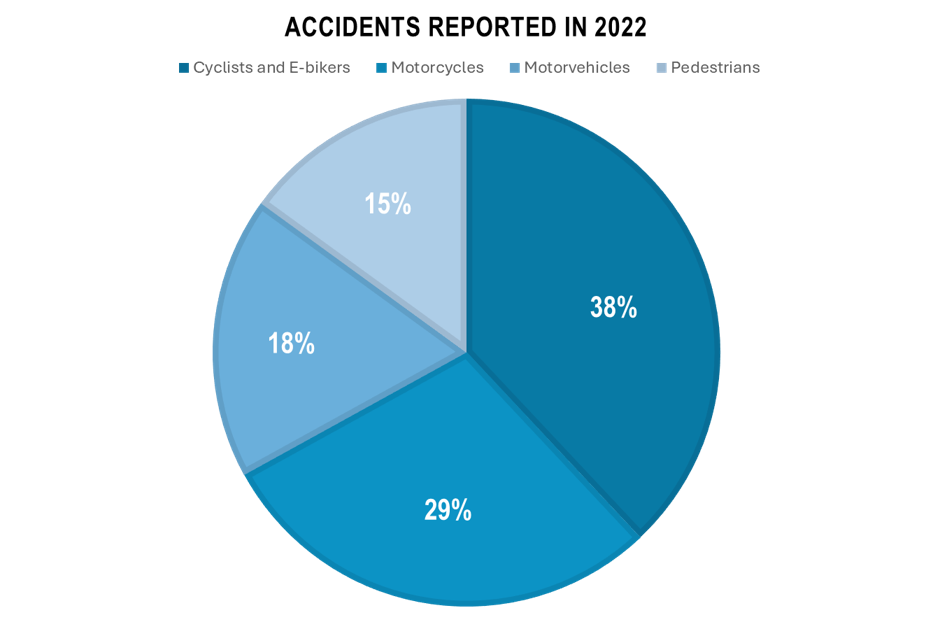
In Switzerland, biking to work is highly encouraged and widely practiced. This is facilitated by the country’s extensive network of bike lanes, bike-friendly infrastructure, and commitment to sustainability However, in terms of safety, Switzerland saw 5,287 cyclist fatalities in 2022, up from 3,793 in 2020. Over the past five years, cycling injuries have increased by 14%, and e-biking injuries have surged by 77%. Meanwhile, incidents involving cars, pedestrians, and motorcycles have decreased.
Irony leading to the aim
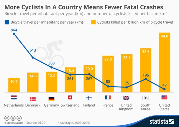
One would think that as the number of cyclists increase the number of cyclists related accidents and bound to increase, but ironically that is not the case, as it can be seen in the graph below the with the increase in the number of cyclists in a country the accidents reduce substantially which can be attributed easily to traffic considerations while designing as well as increased public awareness on road. Thus the need to emphasize increased safety measures and awareness to protect cyclists and other vulnerable road users in urban areas like Zurich where mixed traffic conditions pose significant risks by predicting the severity of accidents at different road junctions.
Aim
Zürich is the largest city in Switzerland and has the highest number of cyclists in Switzerland, with approximately 10% of all trips within the city being made by bike. This translates to over 50,000 daily bicycle trips, highlighting the city’s strong cycling culture and infrastructure. The aim was to predict severity of accidents as classes depending on different features using node classification graph machine learning. The use of node classification was because of dual reasons as nodes are where the maximum accidents occur as well as that is how routes are decided from one node to the other.
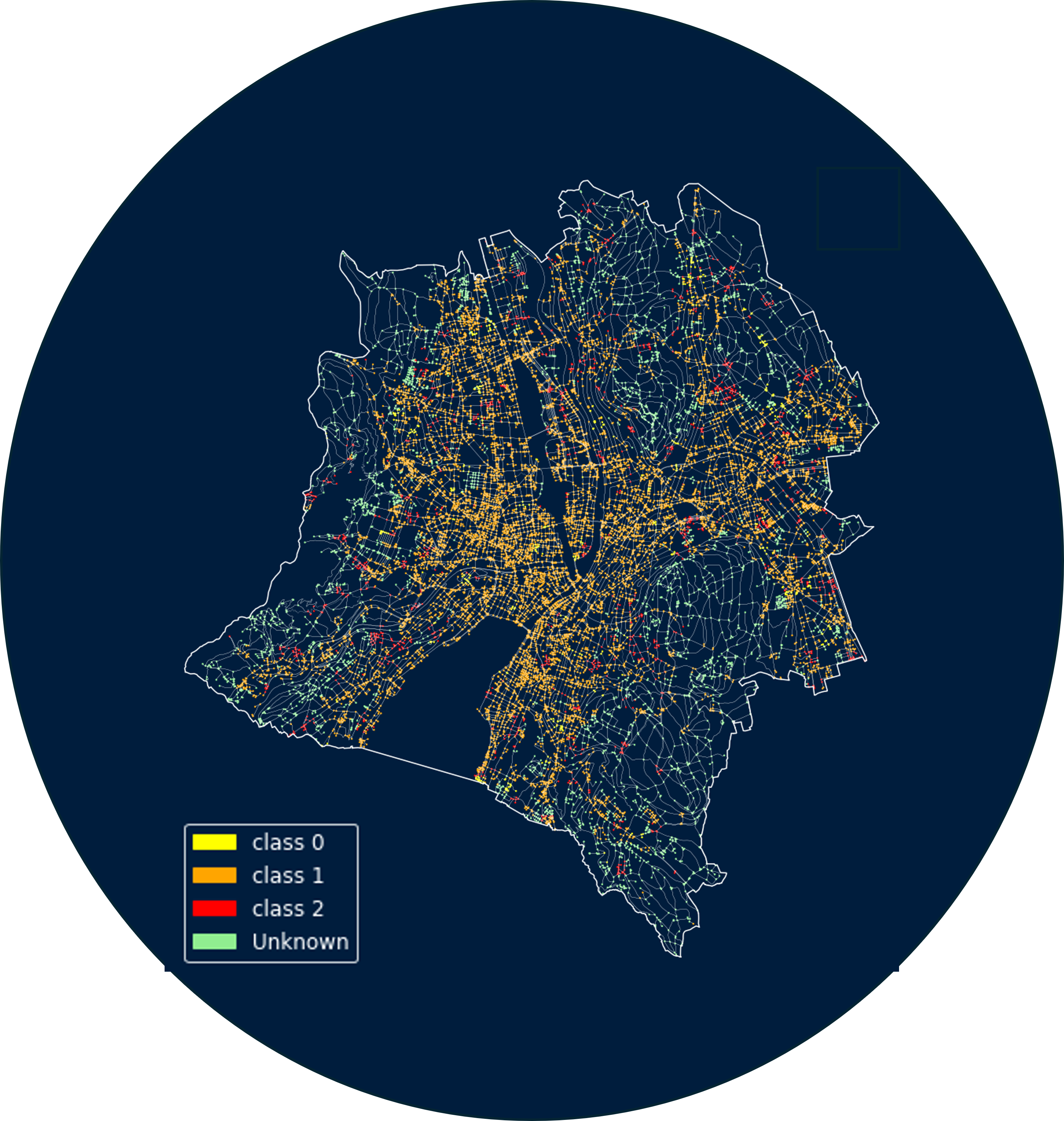
The Figure 3 illustrates the dataset containing of the accident severity plotted the locations of police-registered traffic accidents in the urban area of Zurich and the severity level of it, since 2011.

Graph Machine Learning Aim
The above dataset is added as classes to the nodes which become the labelled nodes (Figure 4) and the aim is to find the classes, i.e. the severity of accidents which can be caused at the unlabeled nodes represented in green.
Class 0: Accident with material damage
Class 1: Accident with light injuries
Class 2: Accident with severe injuries or fatalities
and the Unknown Class is represented by green.
Methodology
Feature 01: Road Noise Pollution Emissions sections
Description: The dataset comprises emission sections delineating road noise pollution within the urban landscape of the City of Zurich as line strings. By integrating road noise data with accident records, a bicycle rider is also aware of the street noise of that bikeway, as cycling is usually done as a tranquil activity rather than just a means of transport.
Hypothesis: As per the initial hypothesis more street noise is a parameter that can be directly co-related to –
- Street Vehicular Traffic
- Pedestrian Rush
- Street Hawkers
- Concentration levels of bicycle riders
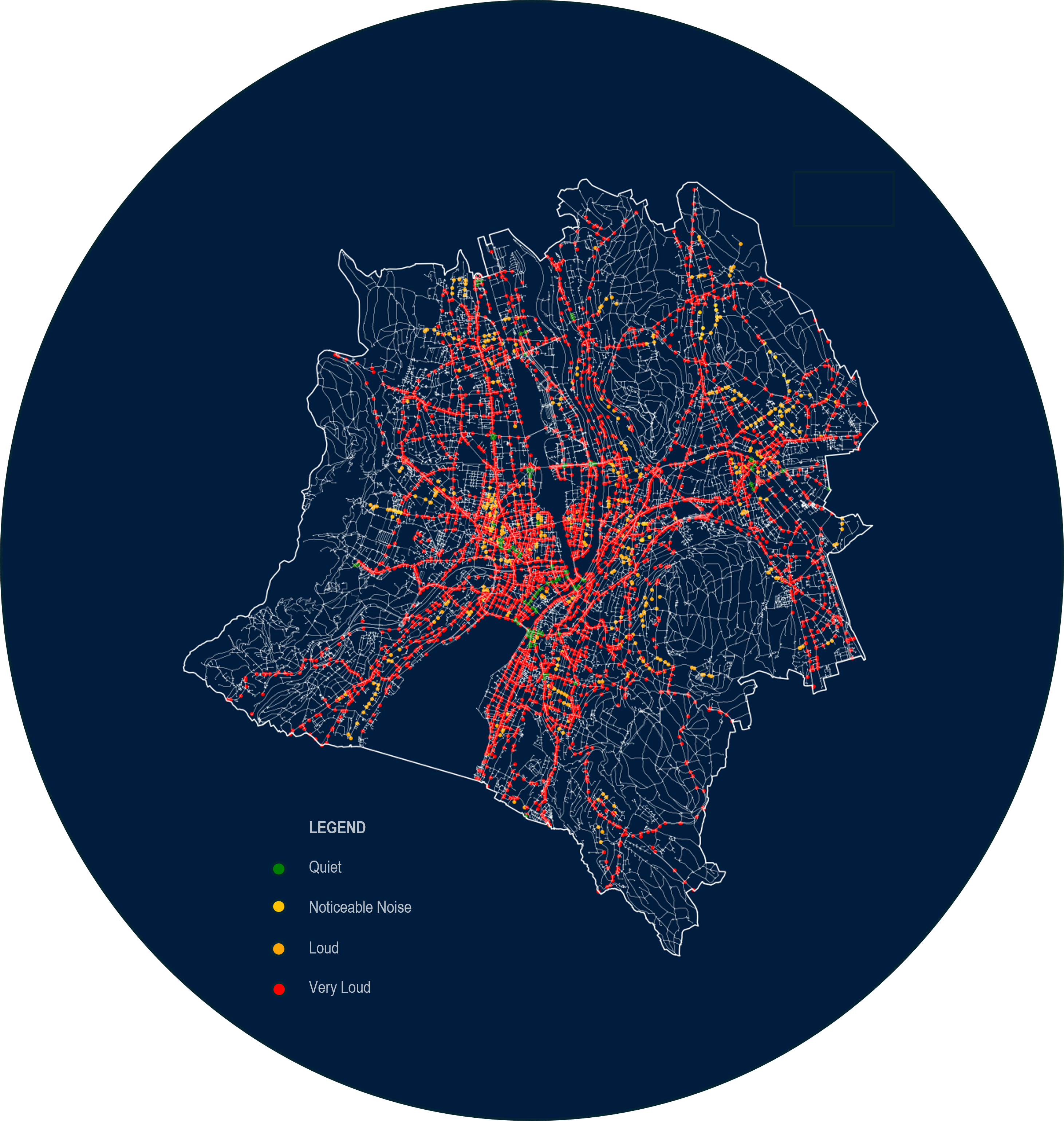
and that is why this dataset was chosen to find out the Unknown Class. Figure 5 represents the color coded line strings to show the noise level from 5 dB to over 400 dB.
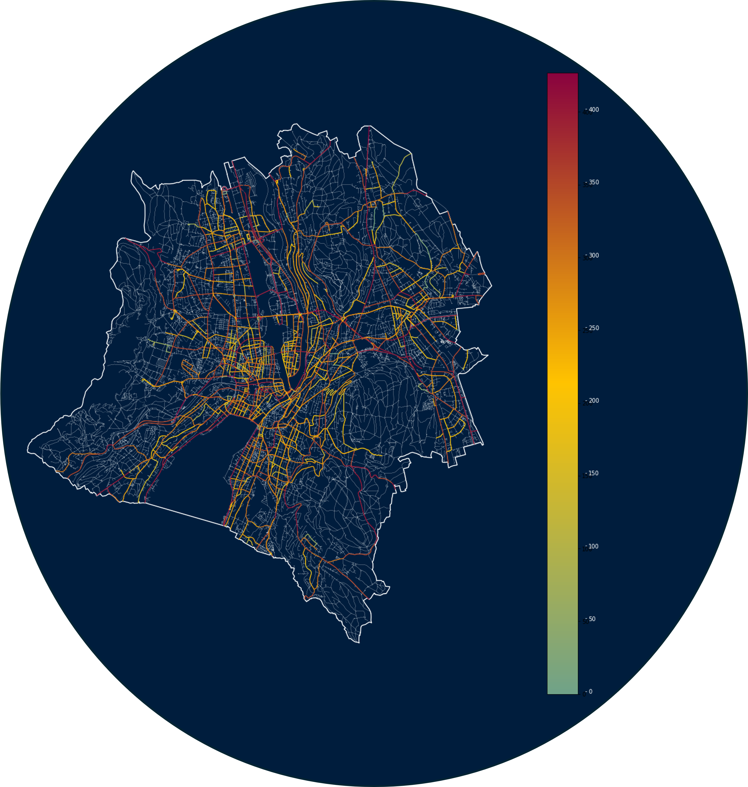
These values are attributed to the nodes to the nodes from the centroids of these line strings using R-tree to find the nearest nodes, the attributes added were as follows
- Quiet Nodes: < 20 dB
- 20 dB< Noticeable Nodes < 40 dB
- 40 dB=< Loud Nodes =< 60 dB
- 60 dB < Very Loud Nodes
Feature 02: Proximity Cluster
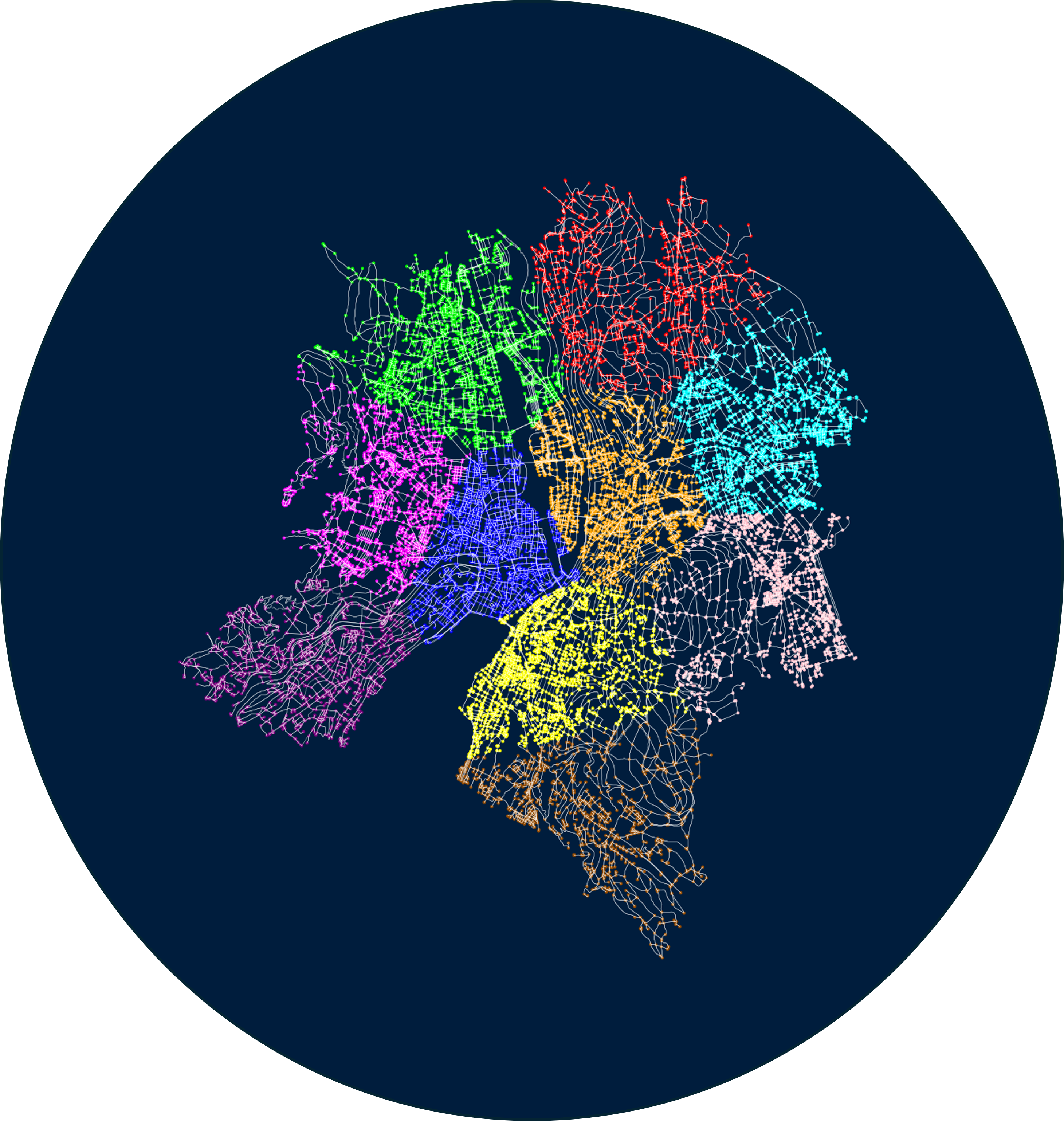
Neighborhood clusters usually have similarities, which is why K-means clustering is used to calculate the proximity index of each node from cluster 0 to 9 and used as a feature to the node. To decide the number of clusters in which the city should be divided, the silhouette core from sklearn.metrics was calculated to be 0.385 for 10 clusters. Any more or less, and the score dropped significantly. This is a good conclusion, as Zurich is divided into 10 districts accordingly.
Initial Training
Co-relation mapping
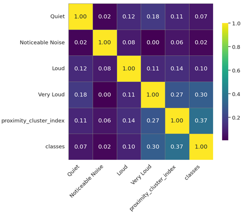
The above two features were chosen for the initial training, before that a correlation heatmap was generated to evaluate the correlation between the features and the classes as seen in Figure 8, from the map we inferenced that proximity cluster index and Very Loud noise attributes shows a correlation with the classes as well as the proximity cluster index as compared to the other attributes, but none of them show a correlation above 0.5.
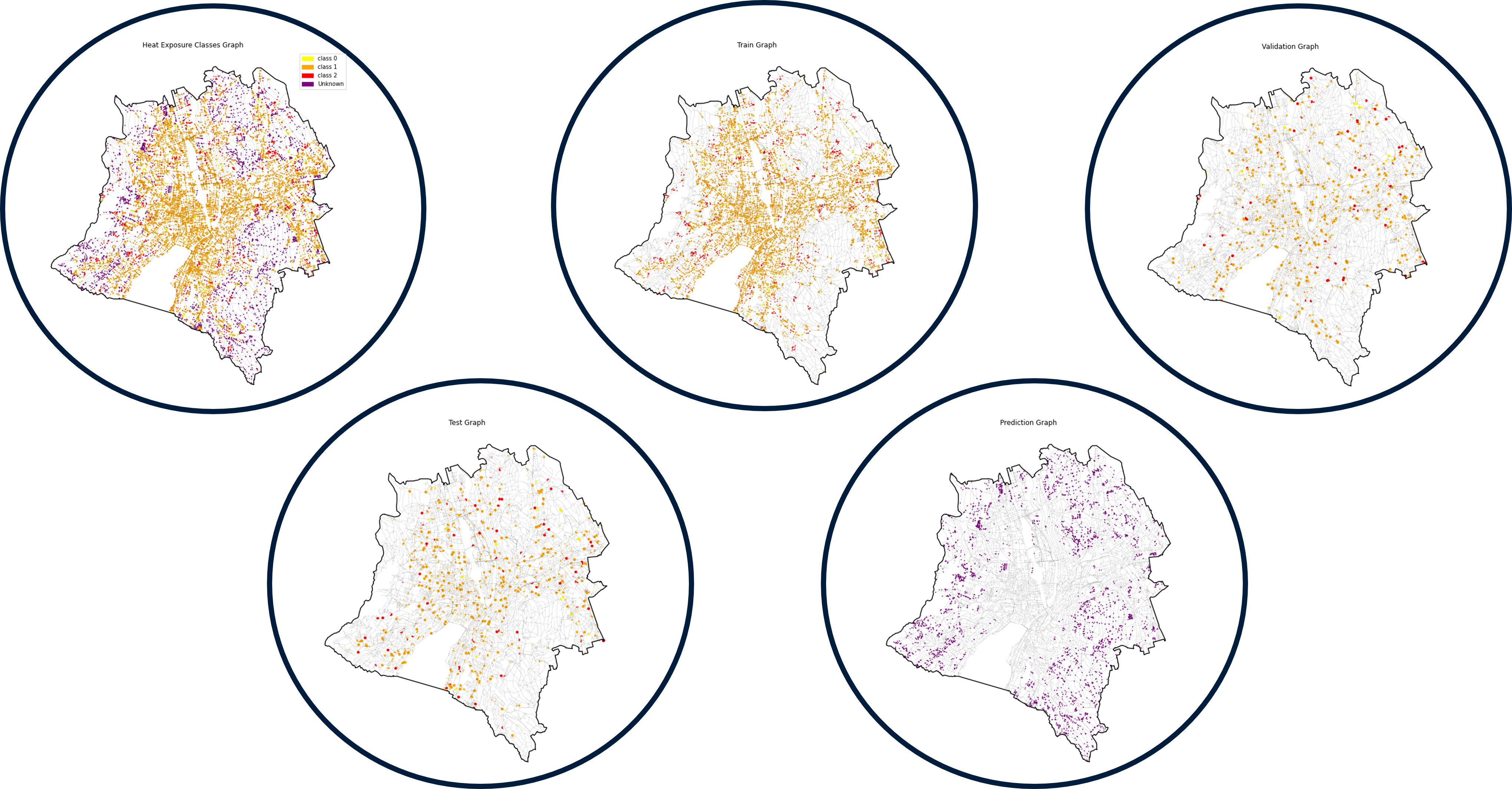
Masking of Labelled nodes
The below figure 9, represents the labelled and unlabeled nodes in part ???.For training, the labelled nodes, they are split into 80, 10, 10 % as train, validation and test nodes , which are the represent in part????, with the last graph representing the nodes to be predicted which are the unlabeled nodes, i.e. the Unknown Class.
Training
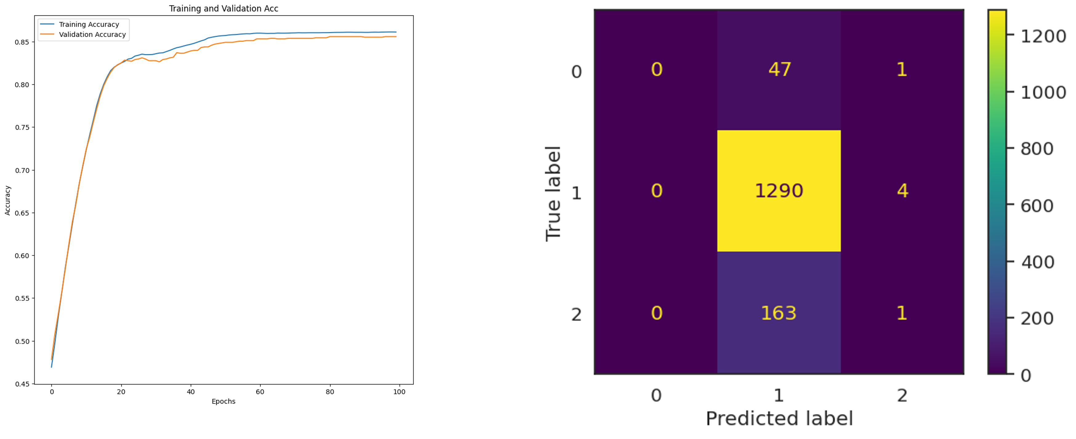
The hyperparameters for training were number of hidden layers =4 ,learning rate=0.01 and n umber of epochs=100 .False Hope: Though the training graph gave an illusion that the training went good as seen in Figure 10.
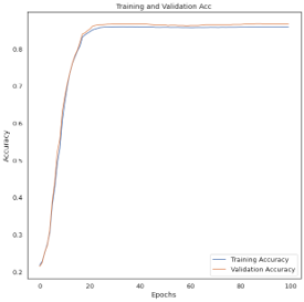
Initial Training Conclusion: From the confusion matrix(Figure 11) it became clear that only Class 01 is getting predicted well while other classes hardly get predicted, and the training graph looked good just because the machine is probably getting trained well for Class 01.
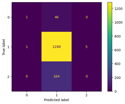
This led to the understanding that probably we we were overestimating the significance of the correlation between noise and severity of accidents, as though practically our hypothesis makes sense but in actuality it wasn’t that simple. Which led to adding more features which have a first layered impact on the pedestrian and vehicular traffic and visibility rather than a double layered one as noise.
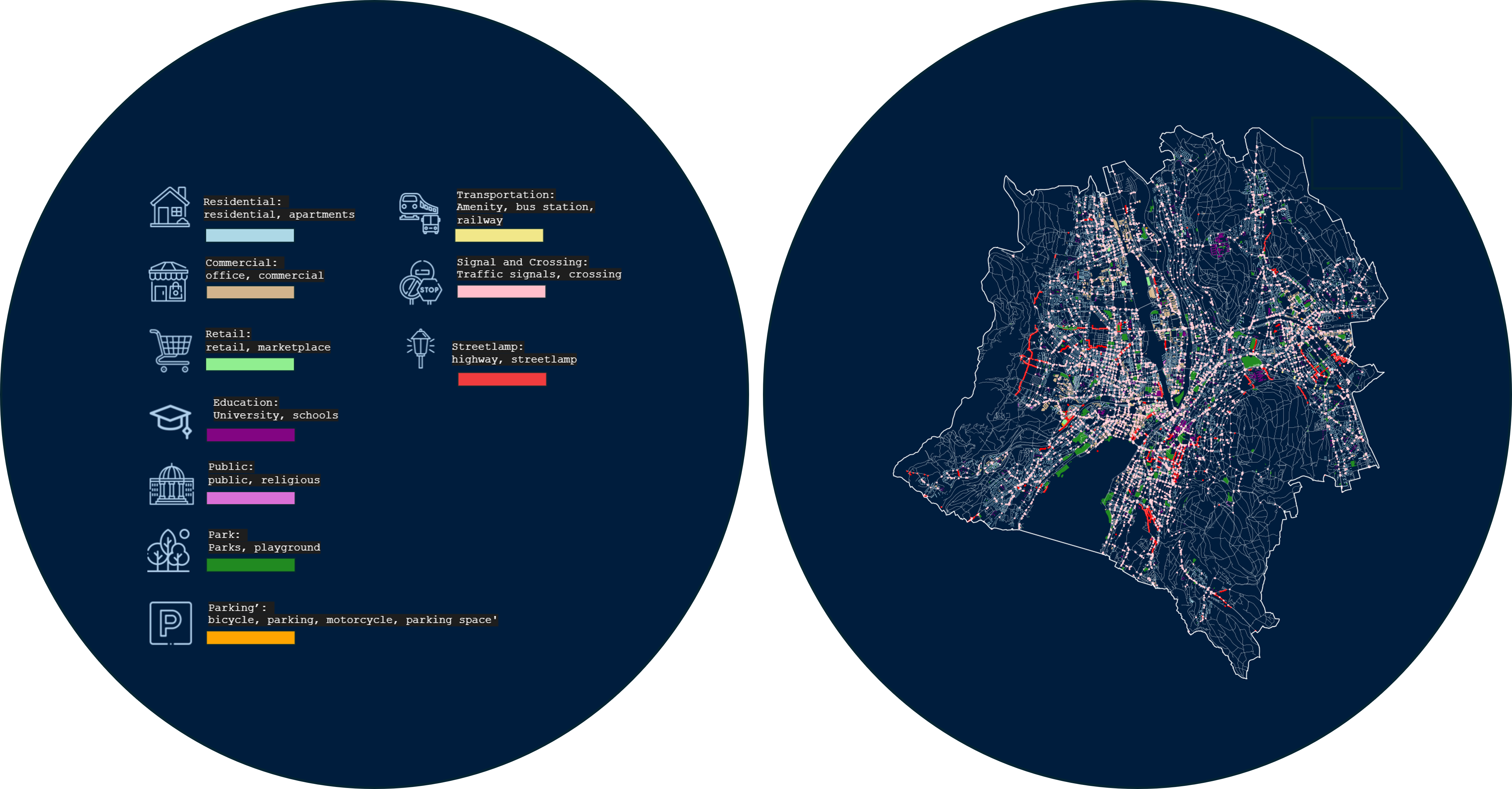
Feature 03 : Hotspots:Building and typologies and route accompanients
As per research, what could be the hotspots of bicycle accidents or undirected crowd mingling as well as road particulars were added from OSM as well as existence and number of signals, crossing and streetlamps all having a direct impact on the severity of accidents.
The features plotted are shown in the Figure 12, The strategy used to transfer this data to the nodes is similar, the centroid of these polygons or points are taken as center points to construct bounding boxes of width 500, and based on the number of times a node has been selected and this data is added to each node as an attribute, this is done because as because of these features the traffic will get affected of all the nearby nodes, these values are normalized before being added as attributes.
Final Training
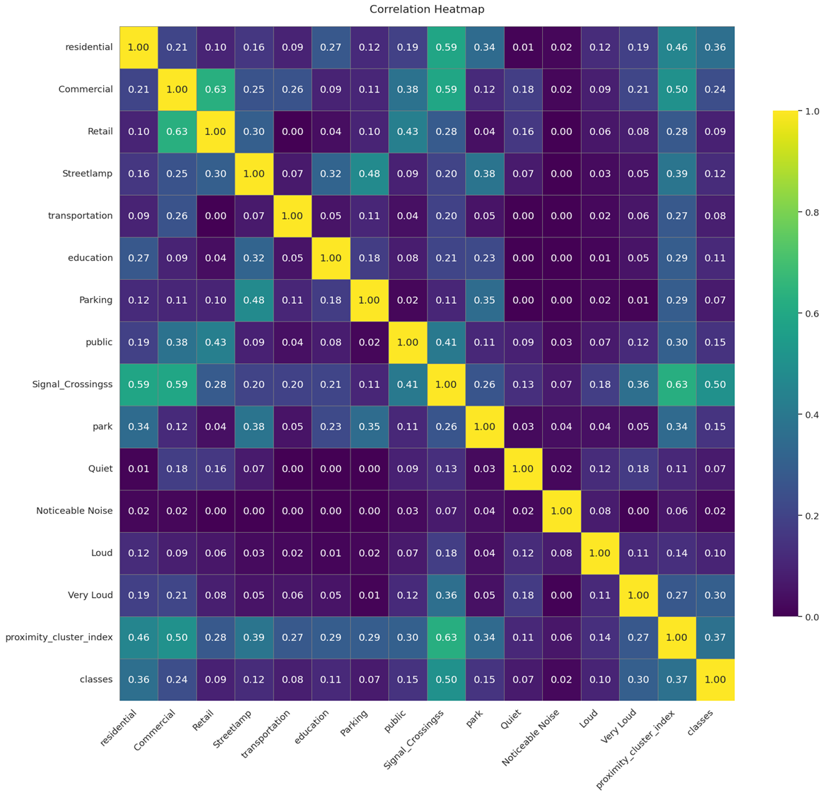
Co-relation mapping
A correlation matrix was plotted to understand all the features relationship with the classes, in which we can see the signals and crossings, along with the residential , very loud and proximity cluster have a better relationship followed by commercial, parks, public building and then the streetlamps.
Training
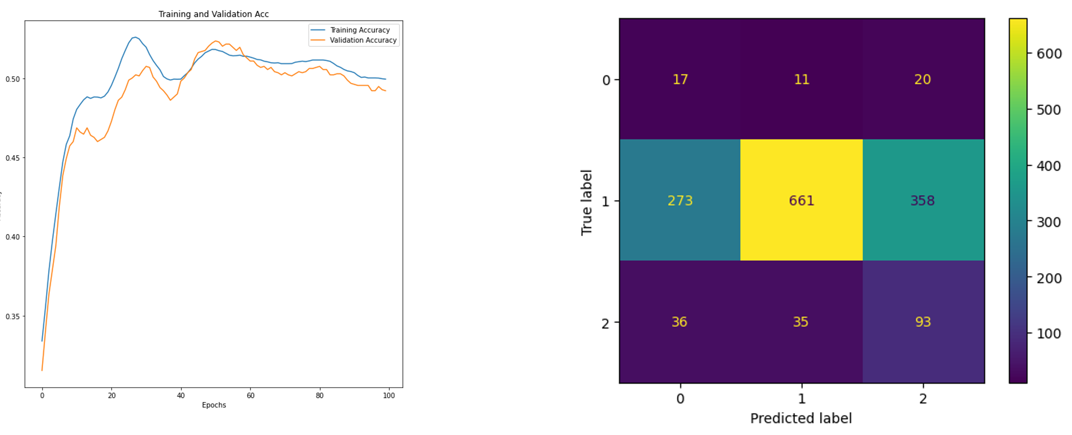
Keeping the hyperparameters same, the model was trained once again, but as it can be that though the training graph looked good, the confusion matrix made it clear that only Class 01 was getting predicted well.
Adding Class weights
Keeping the hyperparameters same, class balancing was attempted to see if the results improve, but as it can be concluded from the confusion matric only Class 01 gets predicted well, the earlier verticality in the graph gets converted to a horizontality.
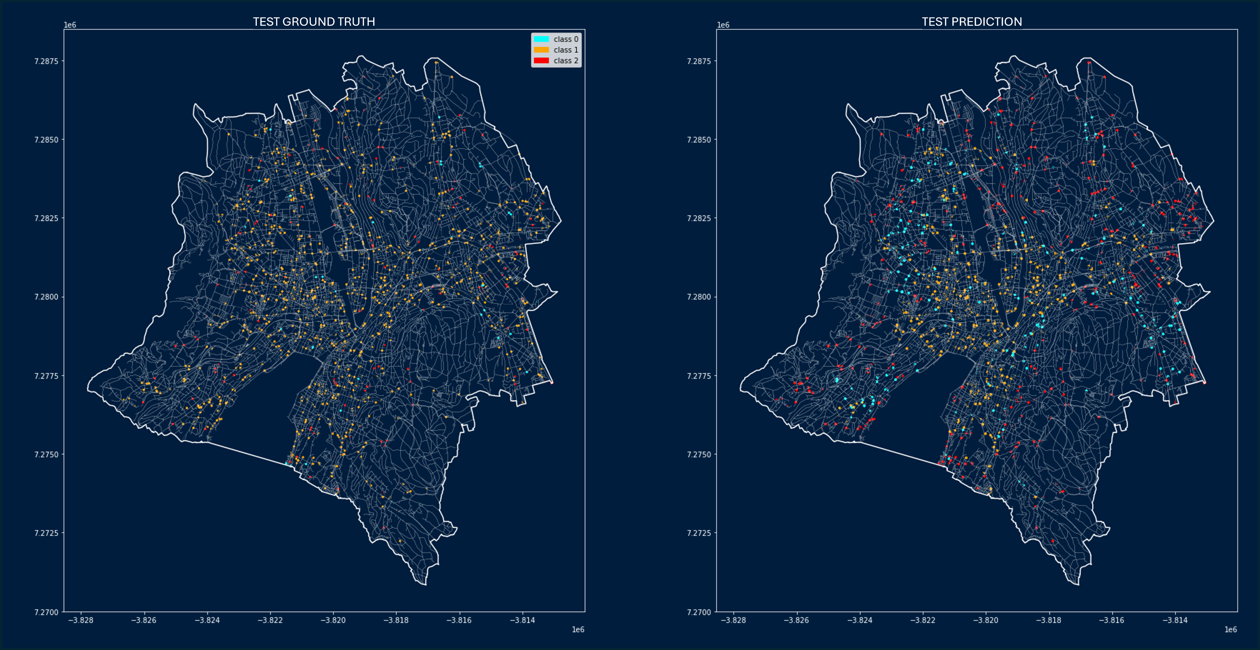
Trained Graph: Testing Ground Truth vs Prediction
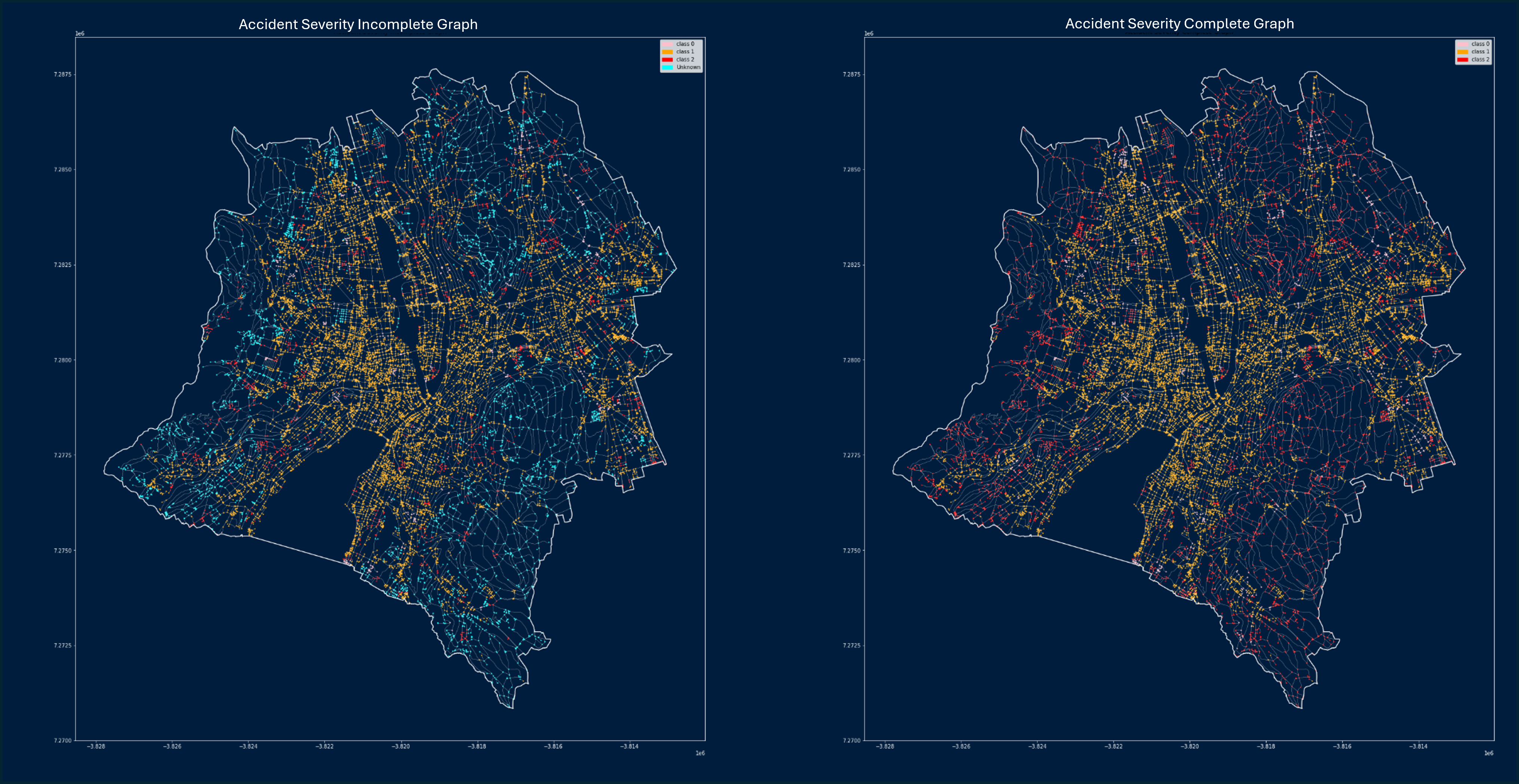
Completing Missing Classes
As can be seen clearly in the figure below most of the nodes get predicted as Class 01.
Conclusion
Class 01 that is Accidents with Light Injuries is predicted well in all scenarios, which can be because of two reasons, the happenstance can be because this class is actually dependent on the features used or it could just be because this Class had the most number of nodes with these attributes.
