From Raw Acoustics to Predictive Insights: Modeling Comfort in Architectural Spaces

Introduction

In this blog, we walk through the complete data science process applied to a unique challenge: predicting the acoustic comfort index of apartment units based on architectural and environmental features. This includes data preprocessing, feature engineering, model training, interpretation, and tuning—with tools like XGBoost, Neural Networks, and SHAP for explainability.

The workflow is split into clear iterative steps, each refining the data and improving model performance. The final outcome not only predicts the Comfort Index effectively but also provides insights into what drives it—a critical step in explainable AI for urban acoustic design.

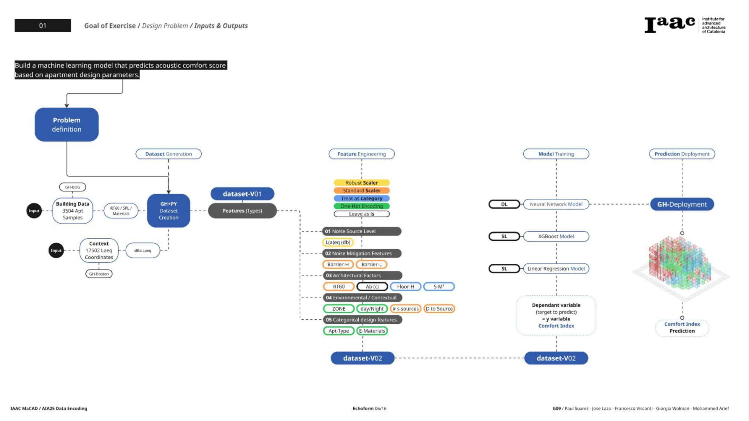
Step 1: Initial Data Exploration and Feature Engineering

The original dataset included both numerical and categorical features—some engineered, such as derived SPL measures, and others raw architectural dimensions.

Key Activities

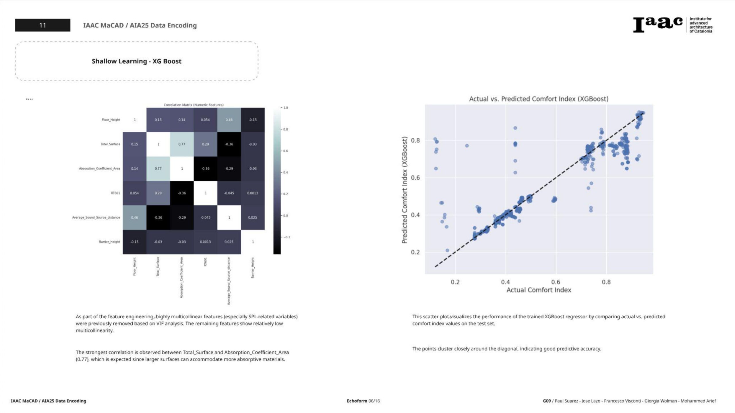
• Initial Pairplots and Correlation Heatmaps revealed strong multicollinearity, especially among SPL features.
• VIF (Variance Inflation Factor) analysis confirmed these issues, prompting the need to remove or reduce redundant features.
• Several derived features were considered for removal in future iterations to stabilize modeling and reduce collinearity.

Step 2: First Major Iteration — SPL Feature Engineering & Advanced EDA

We attempted to harness the predictive power of SPL-derived features by engineering composite metrics.

Feature Engineering

• Created features like:
  • Average SPL
  • SPL range
  • Temporal differences (Δ_SPL)
  • Frequency band interactions

EDA Results

• Correlation Heatmap showed extreme multicollinearity among SPL features.
• Pairplots suggested some clustering by Zone but with overlapping distributions.
• VIF analysis revealed “infinite” values for several SPL-derived features.

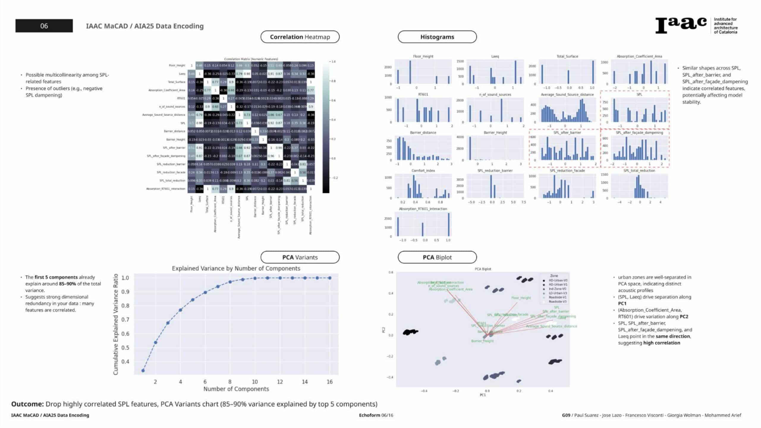
Conclusion

The SPL features dominated the variance in the dataset but introduced serious multicollinearity. We decided to pivot in future steps to focus on core physical and architectural predictors instead.

Step 3: Second Iteration — Refined Feature Selection and Scaling

Here, we reloaded the raw data and focused on a handpicked subset of meaningful predictors.

Selected Features

• Numerical: Floor_Height, Total_Surface, Absorption_Coefficient_Area, RT601, n_of_sound_sources, Average_Sound_Source_distance, Barrier_distance, Barrier_Height
• Categorical: Zone, Apartment_Type, Period
• Target: Comfort_index

Processing Steps

• One-Hot Encoding: for categorical features, with drop_first=True.
• PowerTransformer (Yeo-Johnson): applied to skewed features like Floor_Height, Barrier_distance, and Barrier_Height.
• StandardScaler: ensured all features had a mean ≈ 0 and std ≈ 1.
• Outlier Clipping: applied between the 1st and 99th percentiles.

EDA & Diagnostics

• Pairplot: visualized numerical features by Zone—clearer clusters.
• Correlation Matrix: showed remaining moderate correlations but no critical multicollinearity.
• VIF Check: confirmed that values were mostly below 5; problematic SPL-related multicollinearity was eliminated.
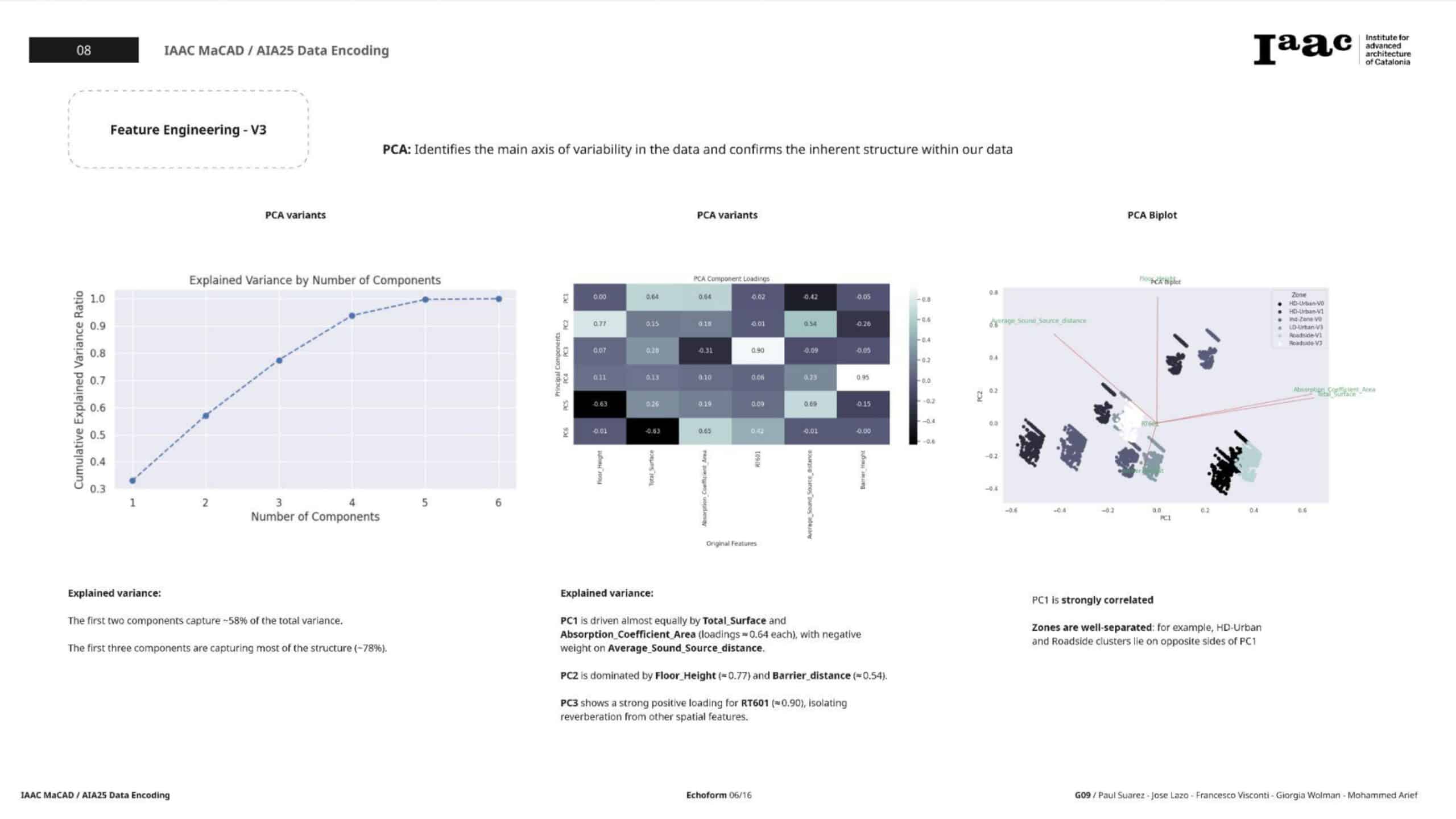
• PCA: helped understand latent structure, with a biplot revealing feature contributions across PCs.

Step 4: Model Training and Evaluation

With the cleaner, well-prepared dataset, we trained two separate models:

XGBoost Regressor

• Train/Test Split: 80/20
• Initial Results:
  • RMSE: 0.0723
  • R²: 0.8800

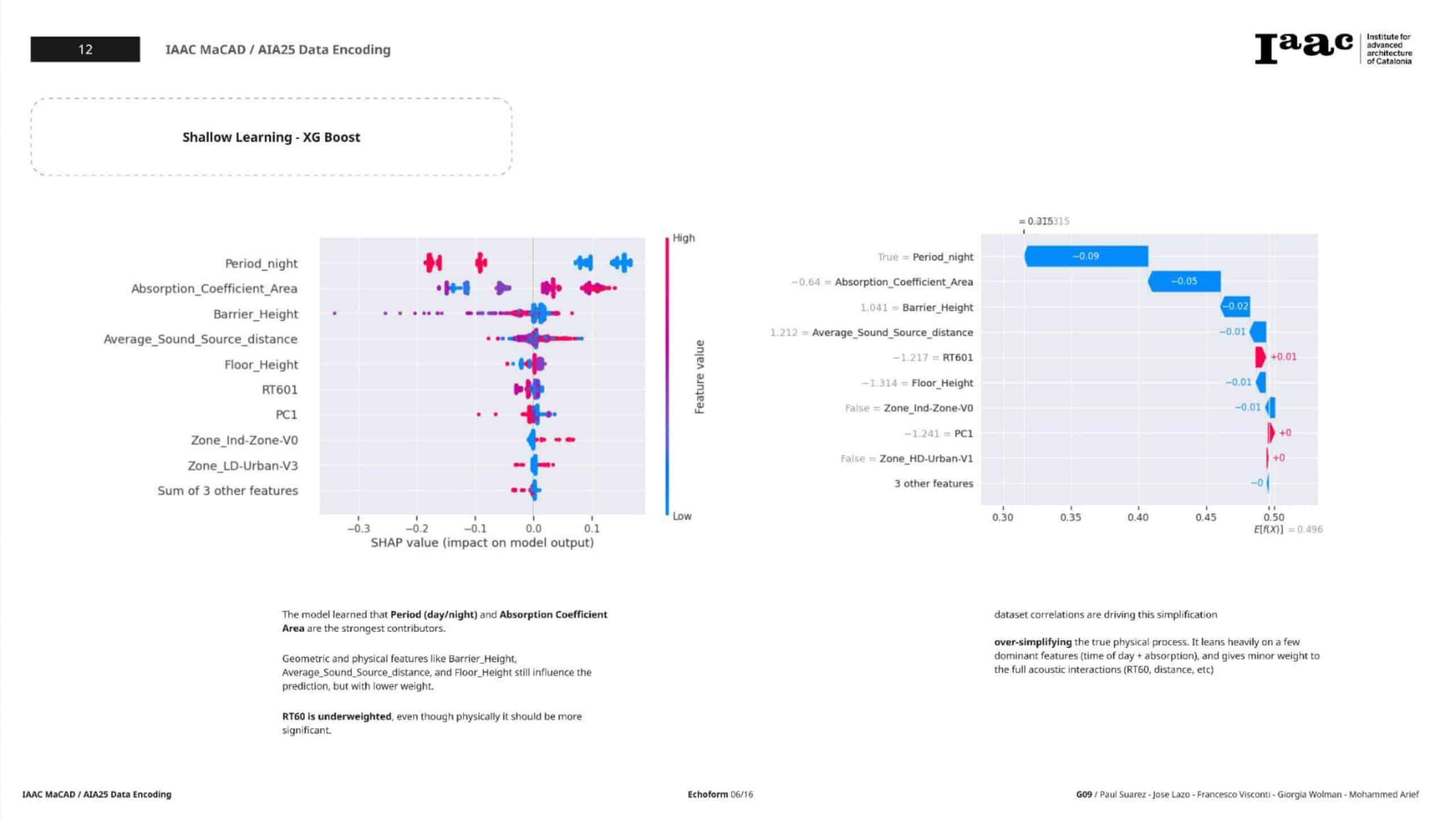
Interpretation with SHAP

• Beeswarm Plot: Identified globally impactful features.
• Waterfall Plot: Illustrated feature-level decisions for individual predictions.
• SHAP analysis added explainability and trust in the predictions.

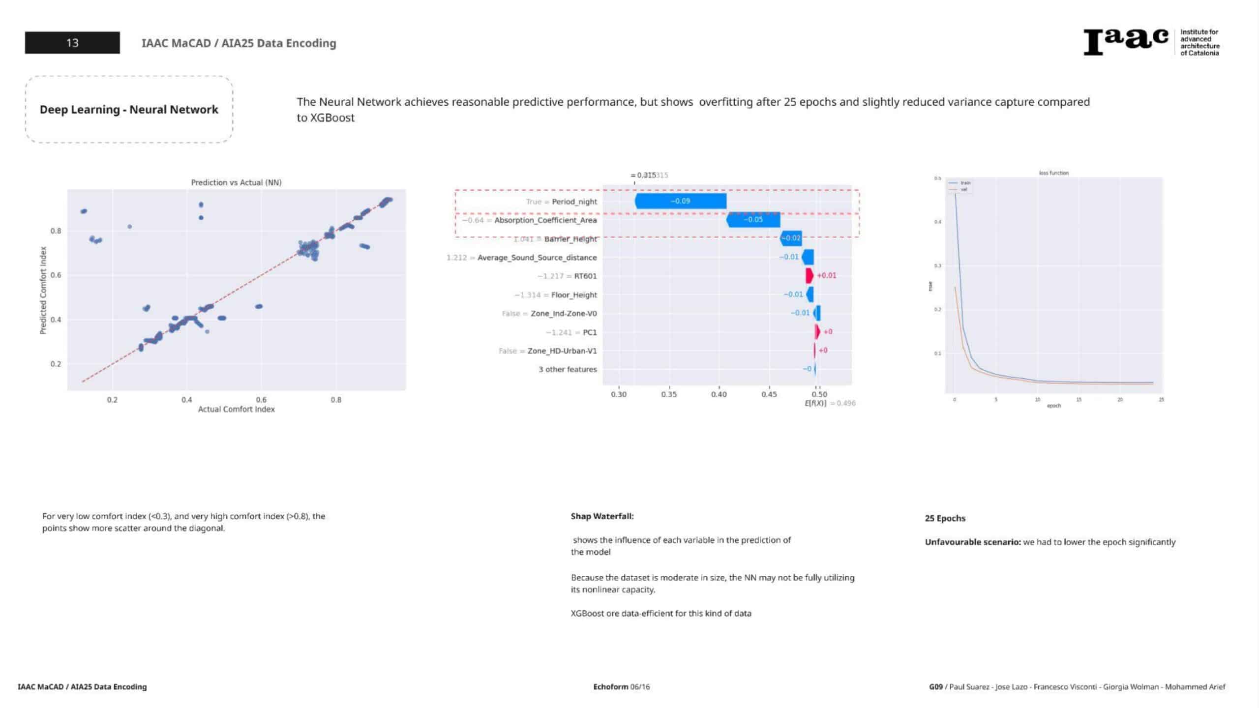
Neural Network (Keras Sequential)

Architecture

• Input layer: input_shape = X_train.shape[1]
• Hidden Layers: Dense(8, relu) → Dense(4, relu)
• Output Layer: Dense(1, linear)
• Loss: Mean Absolute Error (MAE)
• Optimizer: Adam

Training

• Epochs: 30
• Batch size: 64
• Validation split: 20%

Results

• RMSE: 0.0859
• MAE: 0.0330
• R²: 0.8384

Diagnostic Plots

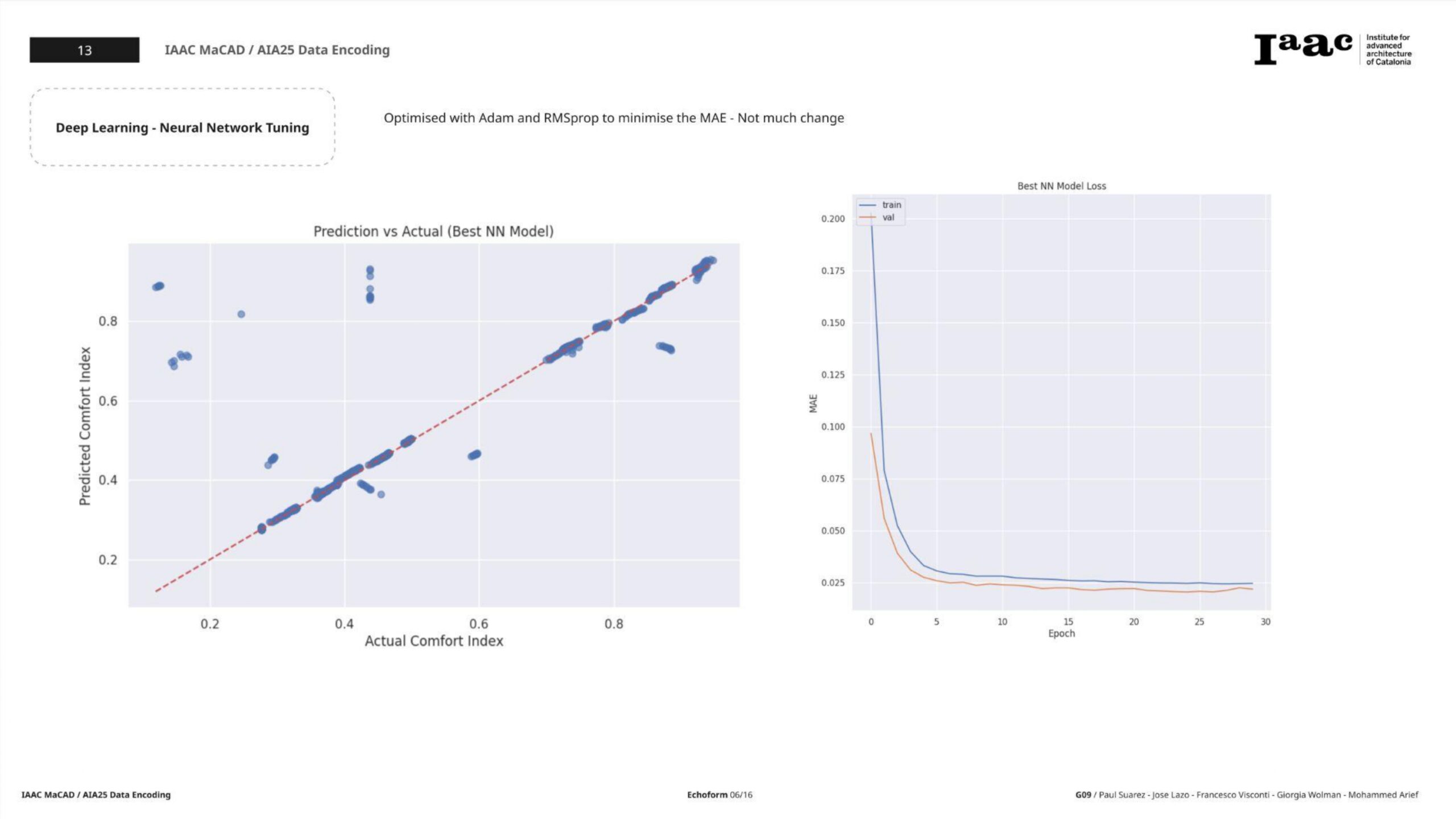
• Loss Curve: Validation loss plateaued → minor overfitting.
• Residual Plot: Most predictions close to the actual values with slight variance.

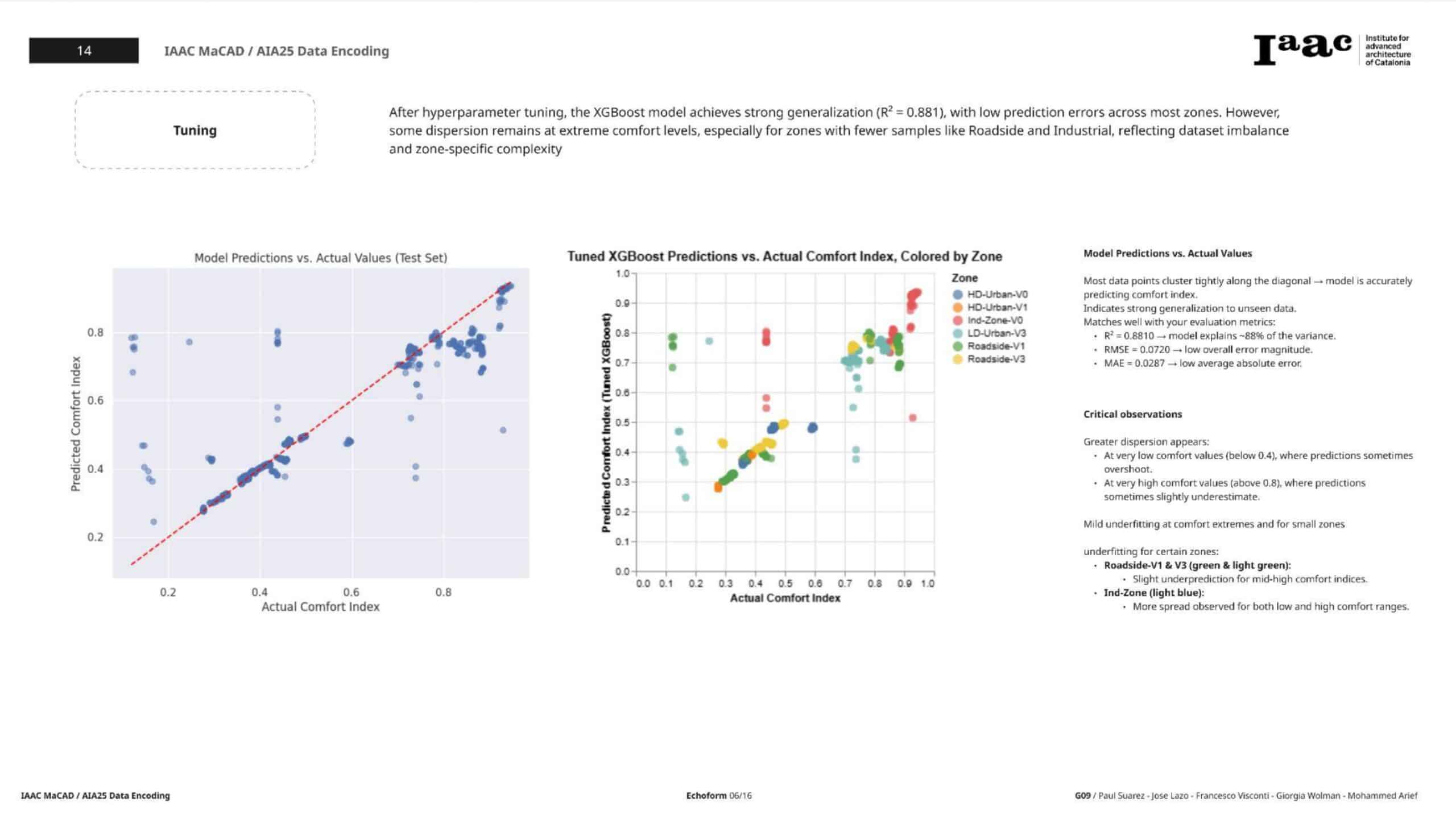
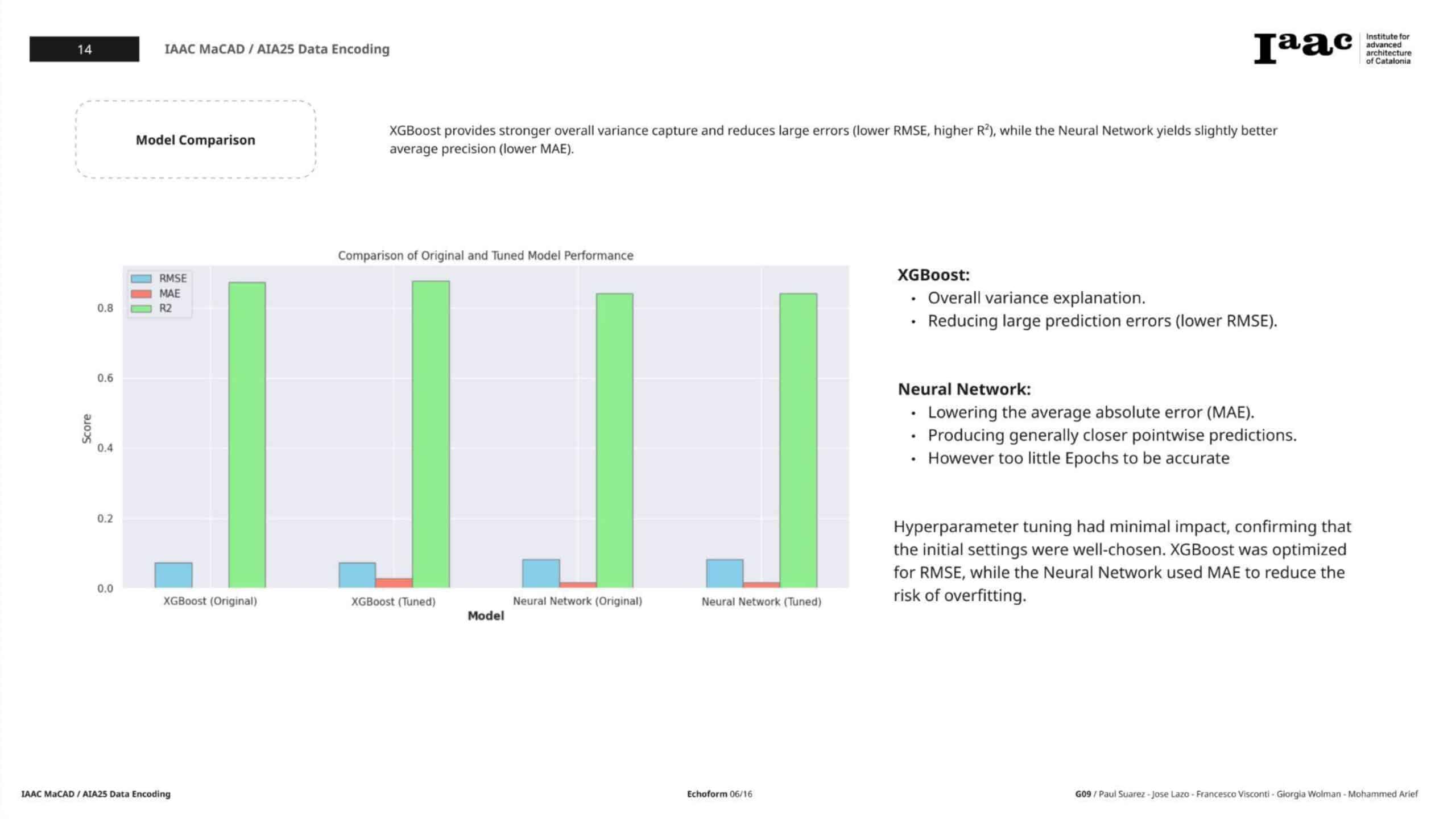
Step 5: Hyperparameter Tuning

To squeeze more performance, we applied hyperparameter tuning via:

5a. XGBoost Tuning (GridSearchCV)

• Grid searched over 108 combinations of:
  • n_estimators, learning_rate, max_depth, subsample, colsample_bytree
• Best Parameters: { 'colsample_bytree': 0.8, 'learning_rate': 0.1, 'max_depth': 5, 'n_estimators': 50, 'subsample': 1.0 }

Tuned Model Performance

• RMSE: 0.0732
• MAE: 0.0288
• R²: 0.8770

5b. Neural Network Tuning (Keras Tuner – Hyperband)

• Searched over:
  • Layers: 1–3
  • Units: 32–128
  • Optimizers: adam, rmsprop
  • Learning rates

Best Configuration Found

• 2 hidden layers
• 64 units in the first layer
• Optimizer: adam, learning rate = 0.001

Tuned NN Performance

• MAE: 0.0201
• MSE: 0.0072
• RMSE: 0.0846
• R²: 0.8356

Final Comparison: XGBoost vs Neural Network

Metric XGBoost (Tuned) Neural Network (Tuned) RMSE 0.0732 0.0846 MAE 0.0288 0.0201 R² 0.8770 0.8356

Conclusion

• XGBoost delivers better RMSE and R²—making it ideal if variance explanation is the goal.
• Neural Network achieves a lower MAE—better for minimizing average prediction errors.
• Both models provide valuable predictive performance, and their combination (e.g., via ensembling) could further enhance outcomes in future work.

Key Takeaways

• Careful feature selection and multicollinearity handling are critical before training.
• Transformations (Yeo-Johnson, Scaling) and outlier clipping improved model stability.
• Model explainability via SHAP strengthened the interpretability of predictions.
• Tuning plays a significant role in maximizing performance.

Future Directions

• Integrate ensemble methods (e.g., stacking NN and XGBoost).
• Deploy the model as an API service or dashboard for architects.
• Explore temporal modeling using time-series if SPL changes are logged over time.

Closing Thoughts

This end-to-end journey from messy, multicollinear data to interpretable predictive models illustrates the power of structured data science workflows in urban acoustic planning. By balancing preprocessing, modeling, and interpretability, we bring AI one step closer to helping humans design better, more comfortable living spaces.