
Daylight autonomy is a climate-based metric that measures the percentage of occupied hours during which a given space receives a specific amount of light, typically 300 lux, through natural daylight alone. It is used to evaluate energy efficiency in building designs by evaluating how much artificial lighting can be reduced throughout the year (Lorenz et al. 154).
This research explores a method for producing real-time daylight autonomy predictions using advanced machine learning, particularly the pix2pix conditional GAN technique. By shifting away from conventional, resource-intensive simulation tools, this approach aims to provide a more efficient and practical solution for predicting daylight autonomy during the early stages of architectural design.
State of the Art
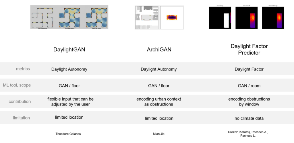
Daylight GAN project was an early initiative exploring the use of CycleGAN for daylight prediction. However, its primary limitation was that the model was restricted to predicting for only one location at a time and did not account for external obstructions. Second, ArchiGAN extended this approach by incorporating urban context as obstructions but remained limited to specific locations. Third, the Daylight Factor Predictor, a previous project developed by us, alongside colleagues Libny and Alejandro during our ‘AI in Architecture’ studio, focused on a different metric—Daylight Factor. Unlike prior projects, which did not emphasize geometric considerations, we aimed to explore various encoding methods for obstructions, such as balconies, not only at the global scale but also at the individual window level to improve model accuracy.
Research Contribution
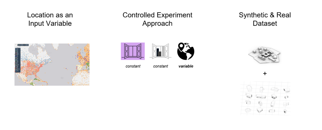
Building on these prior works, we aimed to overcome their main limitation – working with climate data. This thesis contributes to advancing daylight autonomy prediction by introducing several key innovations. One notable aspect is the incorporation of location as a variable input, enabling the model to account for different environmental conditions and climates, unlike previous approaches restricted to single locations. The research also employs a controlled experiment approach, systematically varying room shapes, window dimensions, and external obstructions. This method provides a more comprehensive dataset and allows the model to generalize across diverse architectural settings. Another significant contribution is the combination of synthetic and real datasets. The synthetic dataset includes controlled geometries such as rectangular, L-shaped, and trapezoidal rooms, while the real dataset introduces more complex, real-world building scenarios.
Methodology
1. Dataset: Geometry Generation
For the synthetic portion of our dataset, we used Grasshopper to produce various room and obstruction configurations, aiming for diversity among:
- Room features: Shape, size, and wall configurations,
- Window features: Size, positioning, and frame details,
- Obstructions features: Balconies of different sizes and placements, as well as various surrounding buildings
At the end, we created two sets of geometrical datasets, to explore the controlled experiment approach. In the first dataset, we have 10 thousand configurations, of which 89% make up the synthetic part. In the second one, we have 3,333 configurations, of which 66% make up the synthetic part.
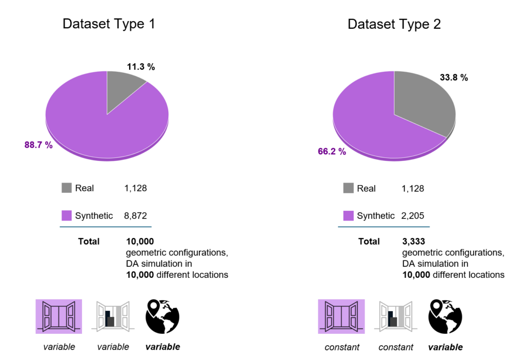
Next, we ran daylight autonomy simulations for both datasets. For Dataset 1, we used 10,000 different geometric configurations, each paired with a unique location. For Dataset 2, we employed a controlled experiment approach, running simulations three times for each geometry with different EPWs (location-specific weather files) to capture their impact on daylight autonomy.
Dataset: Image Encoding
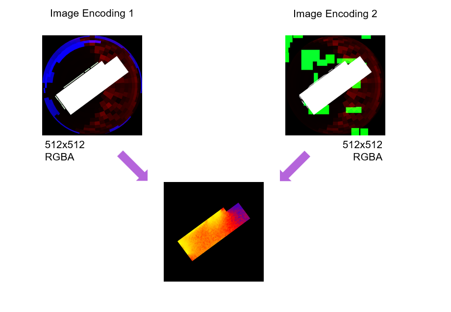
Two methods are employed for encoding the images, and both are PNG images with 512×512 pixel size, utilizing all 4 channels of the PNG images(RGBA).
Image Encoding Method #1
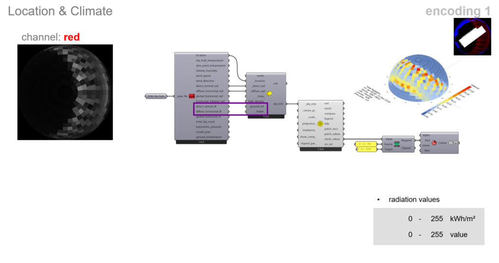
The red channel is used to encode the location information of the room. Here, we are simply using the sky dome component from Ladybug, projecting annual direct normal and diffuse normal illuminance values.
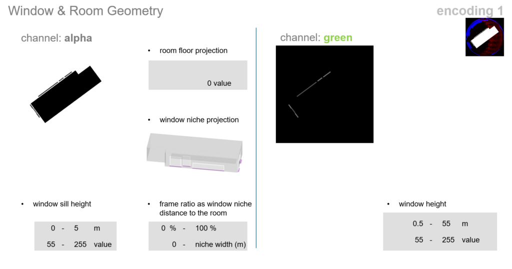
For the window and room geometry of method 1, first the alpha channel is utilized. The room floor is assigned a value of 0, while the window niche is given values between 55 and 255, indicating the window sill height. The frame ratio is represented by the niche’s distance from the room. In the green channel, only the window height is expressed.
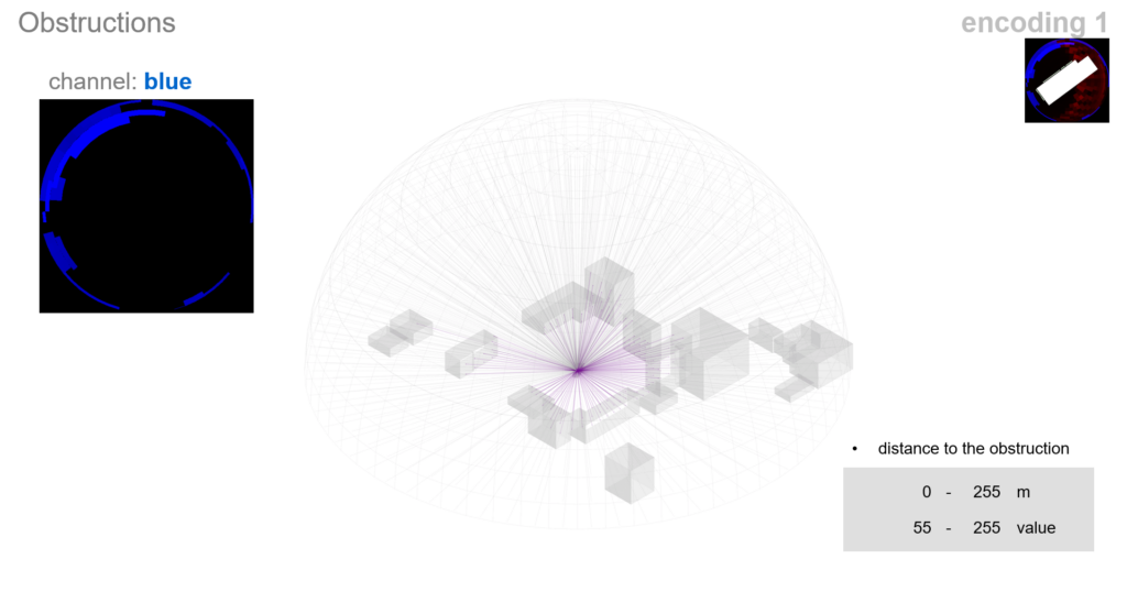
For the obstructions, we are using the blue channel only. Rays are thrown from the center of the room to each patch of the sky dome. Then we compute the intersection points with the obstructions, whether it’s a balcony or a building. Finally, we are encoding the distance to the obstruction in the blue channel, with the exact same scheme for the sky dome.
Image Encoding Method #2
The red channel is used to encode the location information of the room. Here, we are simply using the sky dome component from Ladybug, projecting annual direct normal and diffuse normal illuminance values.
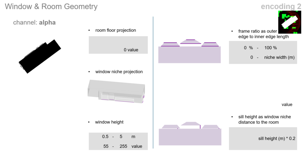
The window and room geometry, are totally packed in the alpha channel. It encodes window height, with the frame ratio and sill height represented by the niche’s scaling and distance from the room floor.
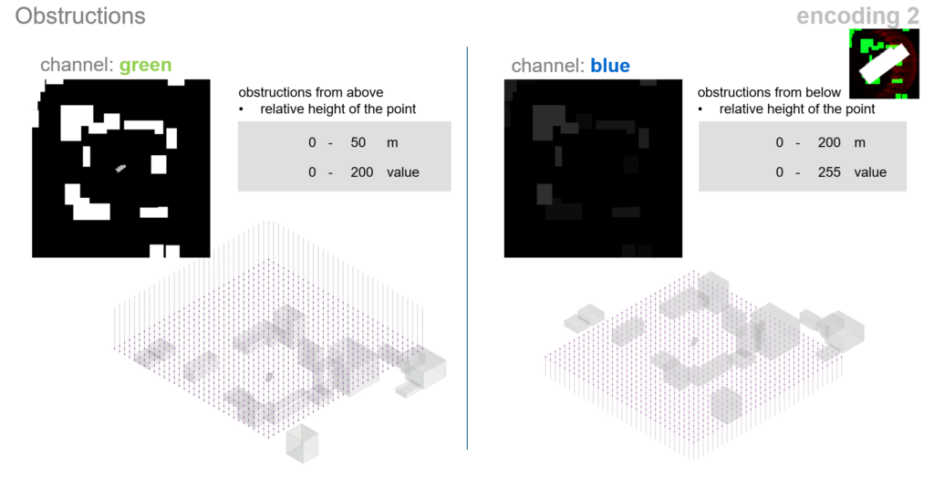
The obstructions are shown in a totally different way. While the green channel encodes the obstructions from above, the blue channel encodes it from below. In other words, we are encoding the height of the highest points of the obstructions in the green channel, and the height of the lowest points in the blue channel.
Model Training
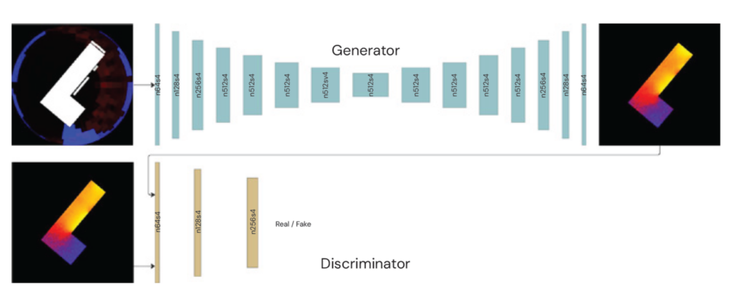
For training, we used Pix2Pix, a type of conditional GAN designed for image-to-image translation, with a U-Net architecture as the generator. The model compresses the input image through 8 layers and decodes it back through 7 layers. We split the data into a training set and a validation set with an 80-20 ratio. After experimenting with various hyperparameter combinations, we found the optimal settings that provided the most accurate results:
•Training and Validation Sets: 80:20
•Batch Size: 4
•Epochs: 35
•Initial Learning Rate: 0.0002
Evaluation
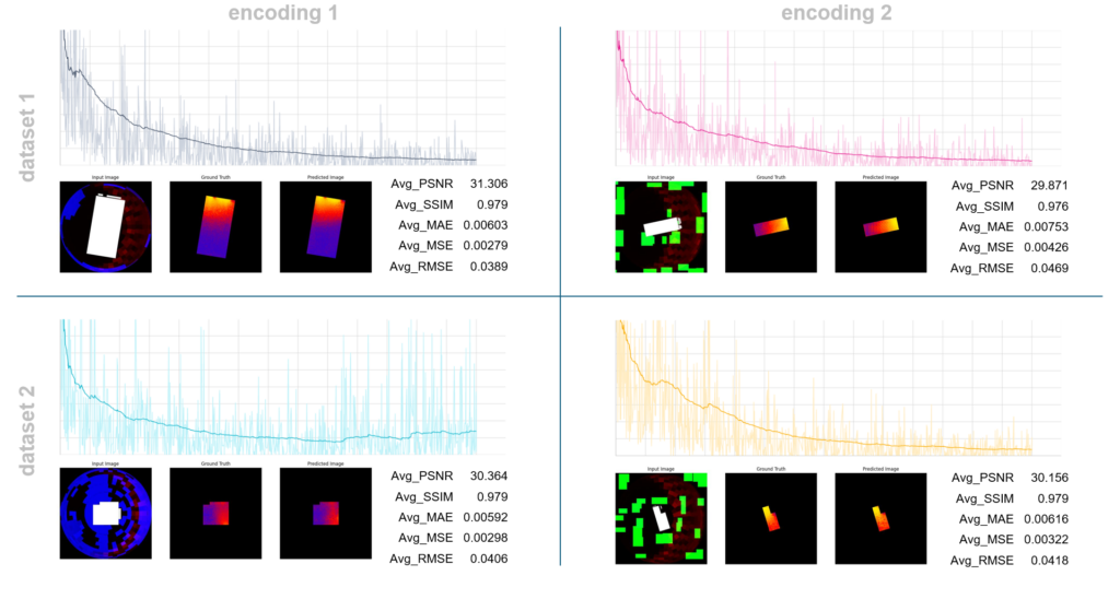
Trainings for 4 cases are done: for two encoding methods and two dataset types. Although the metrics returned similar values, Method 1 produced slightly better results. Additionally, Method 1 was faster to encode in the first place, making it a more favorable option overall.
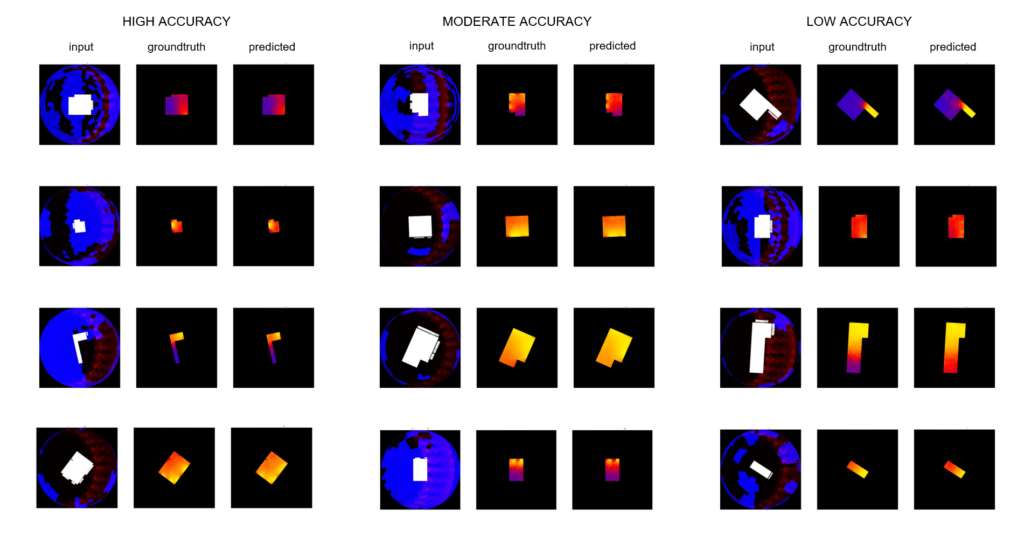
When we have a look at the predictions, we can say that they varied in accuracy, indicating that there’s room for improvement. However, the model successfully captured the distribution of daylight autonomy values throughout the room. And most predictions fell into the moderate accuracy range.
User Interface
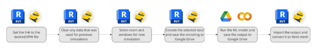
To showcase how our model works, we deployed it in a semi-manual way in Revit 2024 with a custom plugin developed with PyRevit that utilizes Python scripts and Rhino.Inside functionalities. Google Drive was also used as a storage space for the images while Google Colab was utilized to trigger the machine learning model.
The first step for the user is to go to the EPW map and copy a link to a selected EPW file into the popup window. Then the user needs to select room geometry and attached windows that will be used for the simulation. The last part of the process is sending the encoded room to the machine learning model, triggering the script to run it, and importing the result.
Outlook
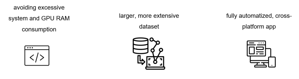
In conclusion, our research demonstrates that it’s possible to teach a Machine Learning model the impact of location input with an adequate encoding and a diverse dataset. What we can improve in our project in the future is system and GPU RAM consumption that limited our ability to use a larger and more extensive dataset, as well as launching a fully automatized cross-platform app for programs other than Revit such as Rhino or ArchiCAD.
