Bits and Pieces

Pictures and symbols are valuable tools to communicate data. Pictures contain input data and representative symbols, generated from points, capture outputs. Pictures, or raster images, are often not geolocated and lack methodological explanation. Here, using the Bitmap+ plugin, pictures of urban conditions are tapped for the data they contain using the coloration of the image and the curves extracted from adjusted and traced raster data. Additionally, symbols take the shape of autonomous agents, typically represented as points or lines, to support legibility of agent movement.

Pictures are used often for the information they contain but not typically as a raw input.

• Curves derived from rasters can be directly imported within Grasshopper as SVGs with the Pancake plug-in. This requires the curve information to be extracted from the raster in an online application, illustration program, or with a code in C++.
• In my experience, the best unique, disjointed curves are generated by bitmapping. The better the bitmap filtering prior to tracing, the better the curve output. Strong advantages were found in images with reflections and varying lineweights.

Pictures programmed randomly can be enhanced when generated and filtered as bitmaps.

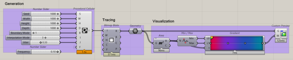
• Procedural cells, fractal pass, and noise can be brought in as vectors using the Bitmap Blobs.
• The extent of an image may be use as the boundary for the generation.

Pictures are powerful storytellers but their imperfect resolution often prevents their use in designing space. The Bitmap+ plugin, developed by David Mans, translates raster images into bitmaps, which contain easily manipulatable then extractable vector geometries and gradient color content. This information can be used to better understand and translate historic maps, hand-drawings, and heatmaps in Grasshopper. In the case of autonomous agents, raster imagery may be translated into the path, obstacle, and force parameters.

Case studies include:

• Space Recognition
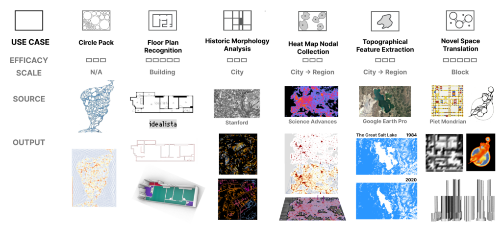
  • Floor Plan Recognition | Idealista | Extraction of 2D curves from architectural drawing to quickly vectorize geometries
  • Historic Morphological Analysis | Nolli Map of Rome | Understanding of block sizes and the relationship between built and unbuilt space
• Extracting Regions of Concern
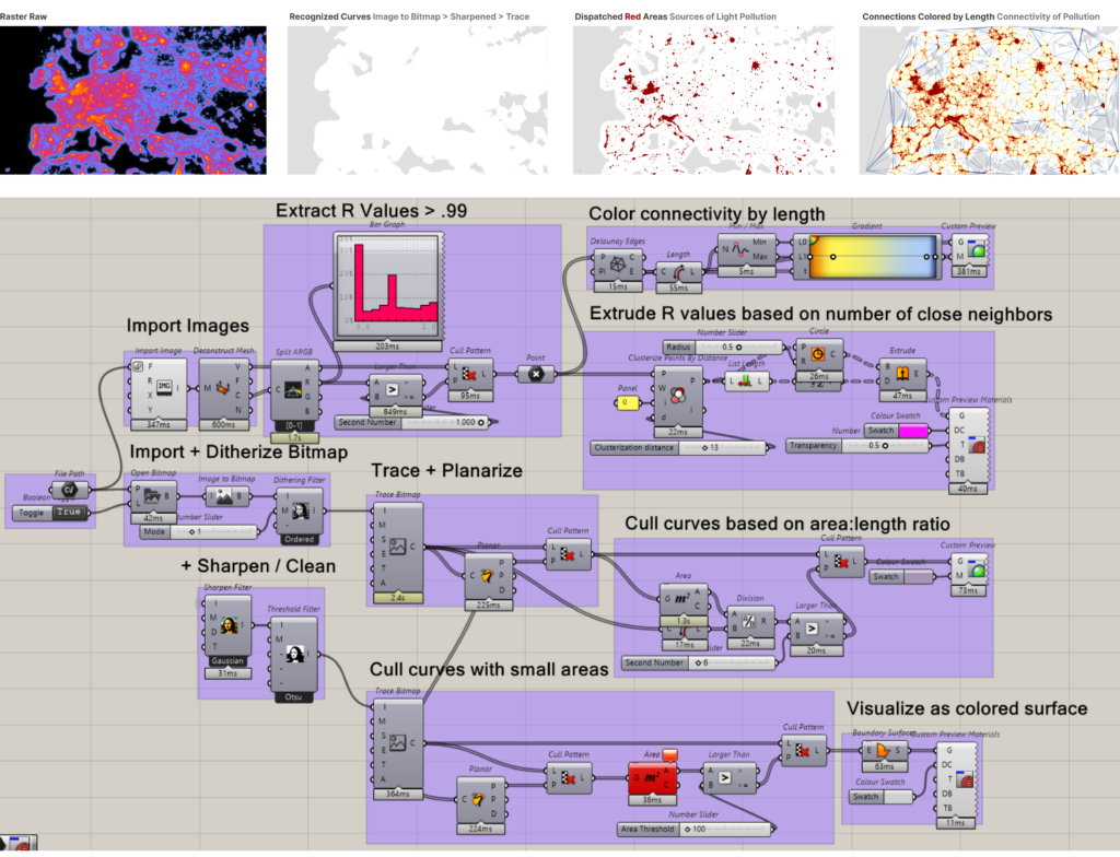
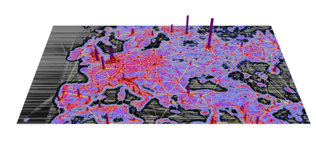
  • Pollution Node Visualization | Light Pollution Map of Europe | Extraction of high R (red) parameter values for risk nodes.
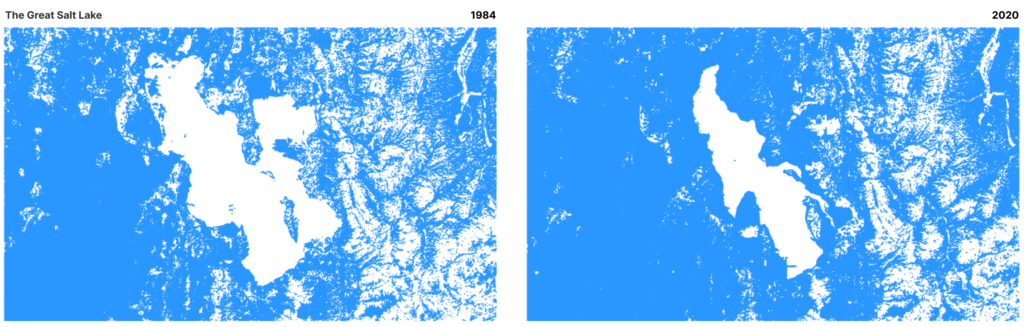
  • Historic Feature Comparison | Google Earth Imagery of The Great Salt Lake | Extraction of high B (blue) parameter values to locate water.
• Novel Space Translation
  • Nested Rooms | Generation of space and optimization of sound source placement
  • Generated Sketches | Categorization and extrusion of novel space
  • Broadway Boogie Woogie | Generation of perceived spaces and understanding of artistic logic

Methodology

Part I: Rasters

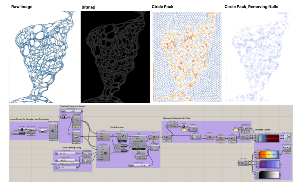
0 | Circle Packing | The study began with an exploration of Kangaroo’s circle packing tool to size circles based on recognize pixel value, and color circles based on their area. This provided an understanding of how raster information can be conveyed through representative geometries.

• Circle packing was found to be computationally intensive even on images of small sizes (~100 MB).
• Lowering the resolution of the image to trace over improves functionality without much impact on the output.
• Using the min/max (extremes) component reduces the number of functions required to program a gradient.

Space Recognition

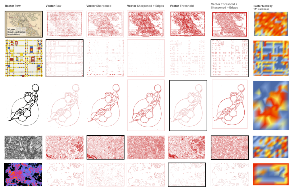
1 | Floor Plan | Reading in Curves | The value of the Bitmap+ plug-in was found by tracing curves with the highest darkness parameter.

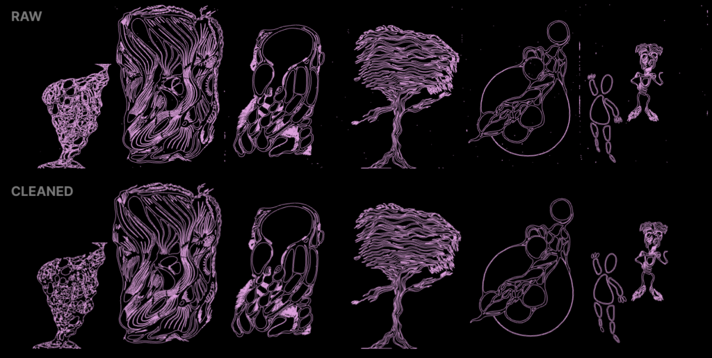
• Culling the curves with the smallest areas cleans the image of noise. This function should be used in all bitmapping adventures.
• A raw trace of the bitmap typically provides the bounding curve of the base geometry as the first list item.
• The threshold filter helps trace the darkest curves.

The value of Bitmap+ filters vary based on the qualities of the input image.

Filters found to be valuable for data extraction include:

• Image to Bitmap
• Trace Curves (Raw)
• Edges > Trace (Construction lines)
• Dithering > Trace (Gradient)
• Sharpen > Trace (For blurry: Reduce noise)
• Threshold > Trace (For faded: Recognize darkness)
• Sharpen > Threshold > Trace (For blurry and faded)

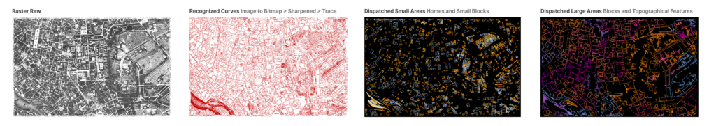
2 | Historic Map | Recognizing Space Types | Space types categorized by area or linearity can be extracted from the bitmapped curves.

3 | Extracting Regions of Concern

3A | Light Pollution Nodes | Sources of pollution and other risks may be identified by extracting the high R (red) parameter values.

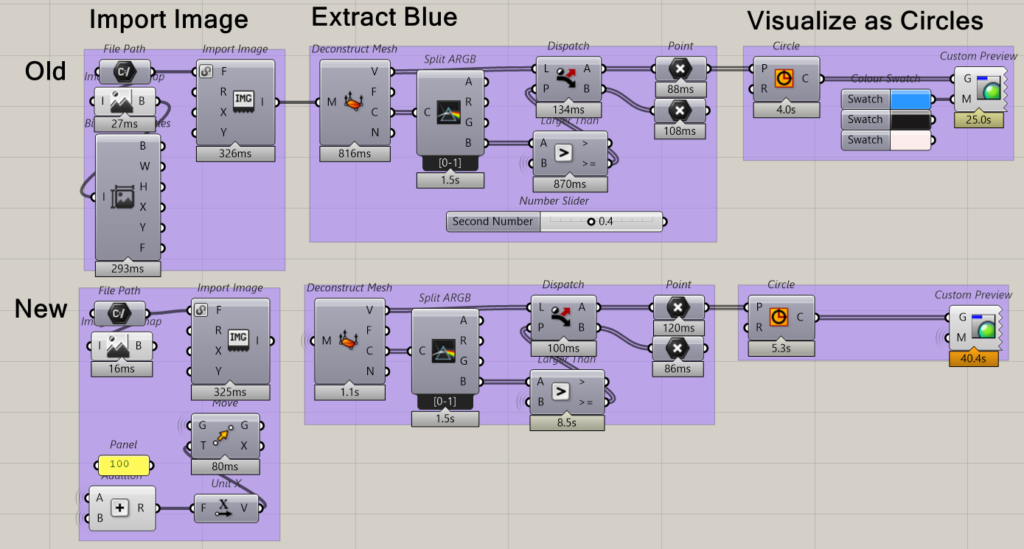
• Bitmaps can be deconstructed for their color properties which map be of interest when filters are applied. That said, importing the image as a mesh and deconstructing it for its color properties is faster.
• Curves often need to be planarized to extract area and length properties and to convert to other geometry types. Planarizing curves often throws an error, which can be ignored. A different method, a cull pattern based on the planar nature of the curve, may be used if non-planar curves are able to be culled.
• The sharpen and threshold filter combination ensures clean extraction of distinct, small areas.

3B | Feature Comparison | Topographical features can be identified and measured for change by comparing historic aerial imagery.

• If comparing similar features, the same zoom should be set when printing from Google Earth.
• This way, the imagery can be mapped with other data.
• Exporting the boundary of the region from Google Earth as a KML allows for geolocation. This can be done by drawing a polygon or placing a point in the center of the image, the centroid of the imported image.
• The image can be bitmapped for its bounding curve to easily access its centroid and scale by its properties.
• To successfully bitmap features of specific color values, images may be taken into photoshop first to extract the feature color within a tolerance.

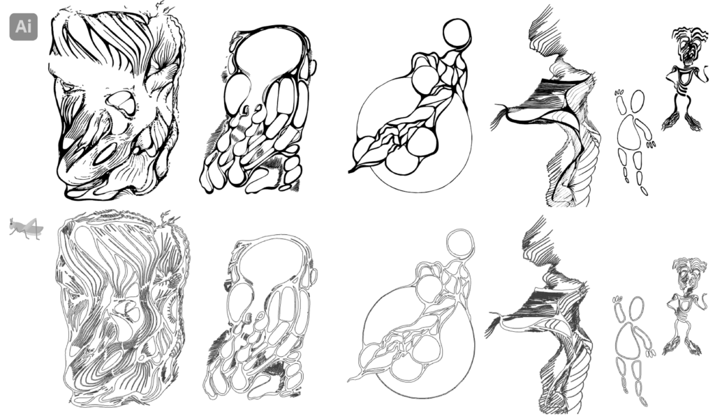
4 | Novel Space Typologies | Hand-drawings are used to imagine space and communicate spatial conditions. But, these drawings are difficult to translate into designs for and data on space. Bitmapping helps extract the key curves in hand-drawings directly to Grasshopper—over plans, on graph paper, and for conceptual purposes to attractor points to simulate movement.

4A | Diagrams can be viewed like layers of trace atop spaces.

• Importing diagrams with the functionality to view their key curves may prove helpful in master plan drafting.
• Overlaying circulation diagrams may support understanding of spaces.
• For a side-by-side view of diagrams, a quick module can be set up in Grasshopper by extracting the properties of the bitmap and moving images by the width parameter of the previous import.

4B | Drawings can be spatialized. Imported in groups, drawings can be analyzed for their common features.

• When working with multiple bitmaps in the same file, it is recommended to add an open bitmap component with a boolean toggle to read in the file.
• If the aim is to loop though the images and ensure consistency in categorization, files paths may be merged and looped through after importing.

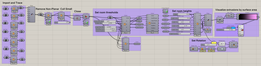
Space Type Categorization | Room types across spaces may be designated by dispatching curves based on area to length then area thresholds. Here, pavilions, linear rooms, large rooms, small rooms, and boundaries are divided.

Agent Placement | After space types are designated, agents can be populated within spaces randomly or in response to room qualities.

1. To place agents at the farthest location from another point in that curve, explode space curves and perform a closest point analysis, inverting the list order.
2. To place agents based on the normalized distance from the wall, construct a mesh colored by the distance from the bounding curve. Then create point groups and select a point as a list item if points should not be within a set distance from one another.
3. To place agents based on the fixed distance from the bounding curve, the wall, offset the curve explode the offset into the number of agents per space.

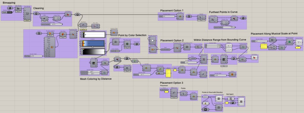
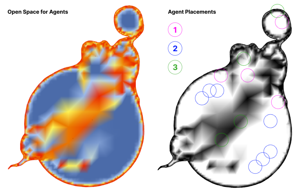
• Dipole placement of agents in circular spaces can be achieve by placing sound sources at points farthest from one another.
• The Pachyderm Acoustic Simulation plug-in would support analysis of agent placement. This would require rendering the space in 3D and baking the model in Rhino.
• To generate multiple agents from a selected source, a random module may be used within the fixed extent of a starting point, along a musical scale, using the cicada package, or at the starting point of an audio wave, using the mosquito package.
• Agents representative of sound can then be moved throughout space using the normalized note value of MIDI data, the peaks and points of MP3 data, or direct MIDI notes from a controller.

4C | Generations

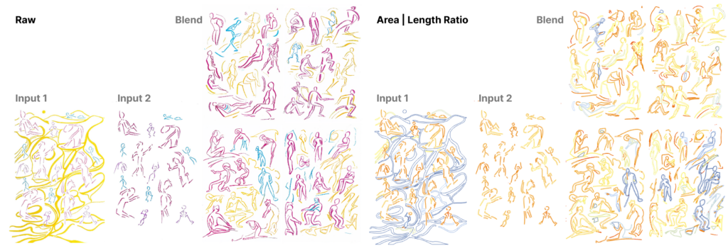
Drawings may also be fed into an image generator such as Midjourney to understand what outputs are generated from specific inputs.

• In this case, the AI seemed to recognize the drawings as those of people and generated new, less abstract people. The connectivity in the first input was not recognized as a secondary layer within the image.
• Analysis can be performed by merging the traced curves and measuring their features. The blended image can also be divided to analyze generations individually.

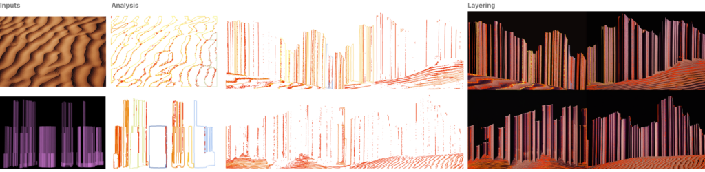
• Generations of blended landscapes have constant properties, those recognized as the relationship between the objects recognized in each image. In the case below, sand dunes are recognized to be the underlying surface for outputs even without a horizon in the image. The extrusions generated in the space type categorization module are recognized to be buildings, extrusions, or rock outcroppings, the linear features atop the dunes.
• Blending the images results in similar outputs because Midjourney is categorizing inputs as layers of space. Variations in generations may be contained within the structure of the inputs.

Part II: Symbols

Symbols are use to categorically represent ideas. In the case of autonomous agents, points that move through fields based on set conditions, symbols may be used to represent different populations, materials, and other points simulated to showcase difference in movement. For autonomous agents to leanly enter and exit loops as point clouds, constructed point geometries, symbols must be generated from single points.

Populating symbolic geometries for populations and solutions supports legibility of agent simulations.

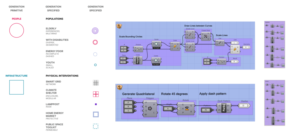
• The simpler the generation of the symbolic agent, the better. Agent simulation is already computationally intense.
• Polygons with variable segments and dash patterns were globally helpful.

Conclusion

The computational flexibility of Grasshopper makes it an exciting tool for visual representation. Raster data can play an important role as an input. Symbols generated from points can improve the legibility of outputs.

Sources

• Interactive Nolli Map: https://web.stanford.edu/group/spatialhistory/nolli/
• Light Pollution Map: https://www.lightpollutionmap.info/
• Food4Rhino
  • Bitmap+
  • Lunchbox
  • Pancake
  • Kangaroo
  • Cicada
  • Pachyderm
• Idealista
• “Rome”, Ratatat