Bridging Carbon estimations in early design stages
The built environment accounts for nearly 40% of global carbon emissions, the urgency to integrate sustainability into architectural and engineering processes has never been greater.
Yet, decisions made in the earliest stages of building design often lock in the majority of a structure’s lifetime carbon footprint, long before traditional analysis tools are applied.
Carbon AI addresses this critical gap by harnessing machine learning to predict the whole life cycle carbon (WLC) of building designs at the early conceptual stage.
By providing rapid, data-driven insights into embodied and operational carbon impacts, Carbon AI empowers architects, engineers, and developers to make informed, sustainable choices from the outset.
This proactive approach not only accelerates low-carbon design iteration but also aligns with emerging regulations, green certification standards, and corporate ESG goals.
” With Carbon AI, sustainability becomes a core design parameter and not a post-design adjustment.”
——————————————————————————————————————————————————————————————————————————-
Structure
What is under the hood?
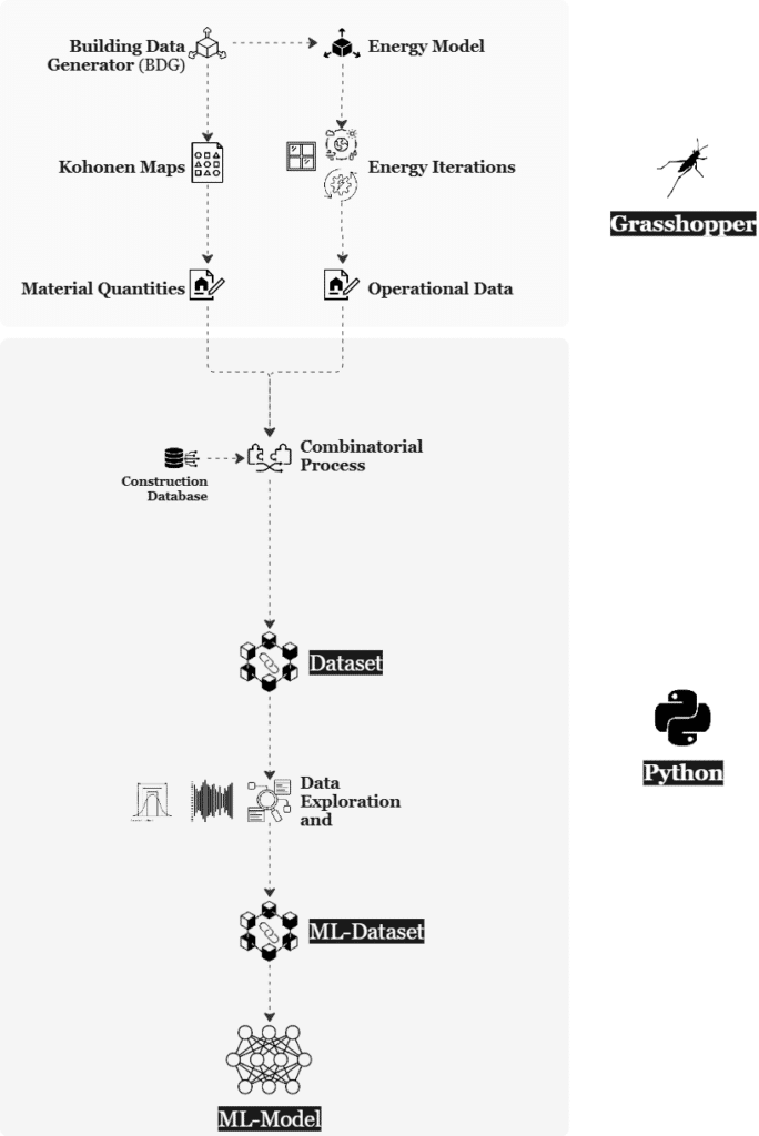
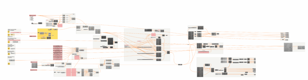
This workflow illustrates a complete data-driven pipeline for evaluating building performance and environmental impact, integrating parametric modeling in Grasshopper with data analytics and machine learning in Python.
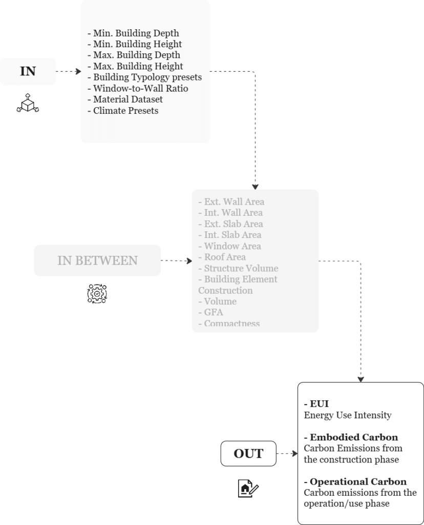
It begins with a set of input parameters such as building dimensions, typology presets, window-to-wall ratios, material databases, and climate presets. These inputs are processed through the Building Data Generator (BDG) to create diverse design scenarios. In the in-between phase, the system calculates intermediate attributes, like wall areas, slab areas, structure volume, window and roof areas, gross floor area (GFA), and compactness, which form the geometrical and construction basis of each building variant.
These characteristics feed into a simulation engine, where Energy Models and Energy Iterations estimate performance under various conditions. Simultaneously, Material Quantities and Operational Data are generated. From these, key performance metrics are derived:
- EUI (Energy Use Intensity) for operational efficiency,
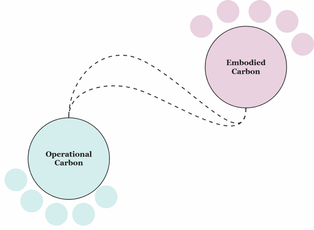
- Embodied Carbon, representing emissions from construction materials, and
- Operational Carbon, indicating emissions during the building’s use phase.
The data then passes through a Combinatorial Process, integrating with a Construction Database, resulting in a comprehensive Dataset. In Python, this data is explored, refined, and transformed into a structured ML-Dataset, which is used to train a Machine Learning Model. This model can predict performance outcomes and support design optimization, closing the loop between environmental goals and architectural design..
——————————————————————————————————————————————————————————————————————————-
Dataset
Where does the information come from?
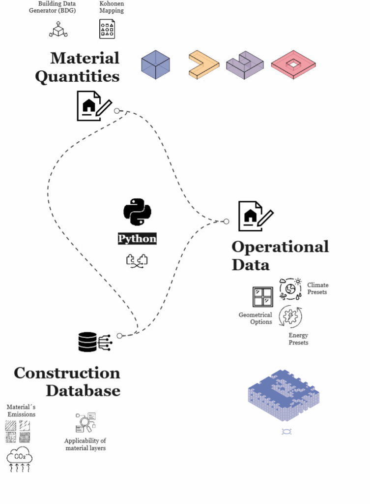
The dataset creation relies on three sequential pipelines that merge into one. Initially, a material database with environmental data for common materials was created. Then, on the geometrical side and based on a common building data generator, materials quantities are acquired. Lastly, these geometries are fed into an automated energy simulation loop to produce the rest of metrics necessary for obtaining the complete dataset.
The animation below shows the different iterations during the energy simulations.


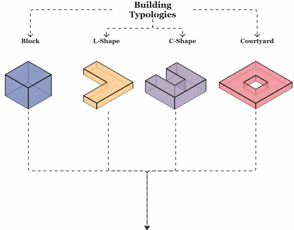
The whole concept is conceived for Residential typologies such as blocks, L-, C-, and courtyard-shapes. Which were created by employing Kohonen Mapping. This way, a well balanced geometry dataset was created.

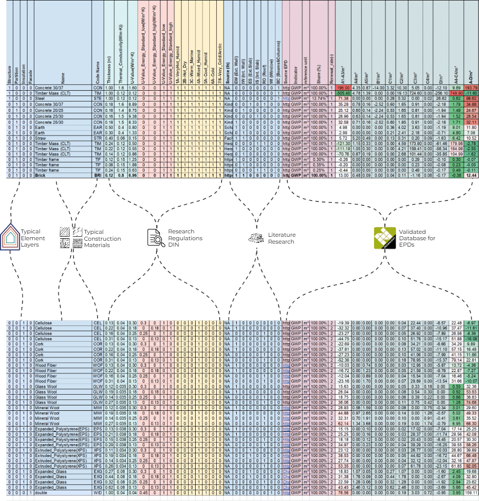
An exhaustive literature- and web-based research about material properties for different climates and their applicability to different building elements was essential. For instance, we used Okobaudat, a validated database for EPDs, to obtain the relevant GWP data for the creation of our dataset.

Lastly, all combinations iterate in an automated energy simulation approach, providing the necessary metrics for operational carbon calculations.

——————————————————————————————————————————————————————————————————————————-
Data Handling
How does the dataset look like?
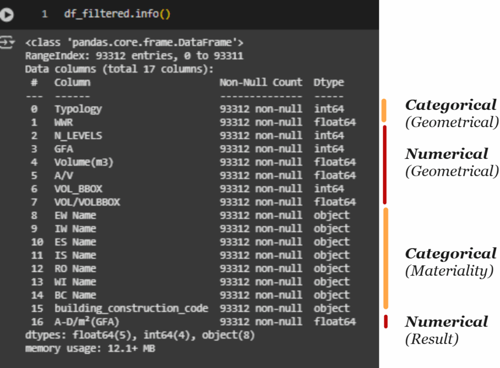
Our dataset started with 71 features, then we manually reduced dimensionality to focus just on the most informative ones (17 Features).
The second part of the workflow focuses on how building performance data is structured and prepared for machine learning in Python. The dataset, shown in the first image, contains over 93,000 entries and 17 features, which are grouped into three categories based on their role in the analysis.
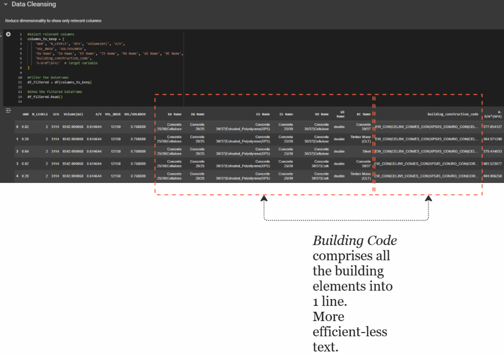
Geometrical features include both categorical and numerical variables, such as building typology (Typology) and metrics like gross floor area (GFA), volume, and aspect ratios. Material attributes, such as wall and roof types, are treated as categorical variables and are represented as object types in the DataFrame. Finally, the dataset includes a numerical result, specifically A-D/m²(GFA), a performance metric that represents whole life cycle carbon intensity per square meter.
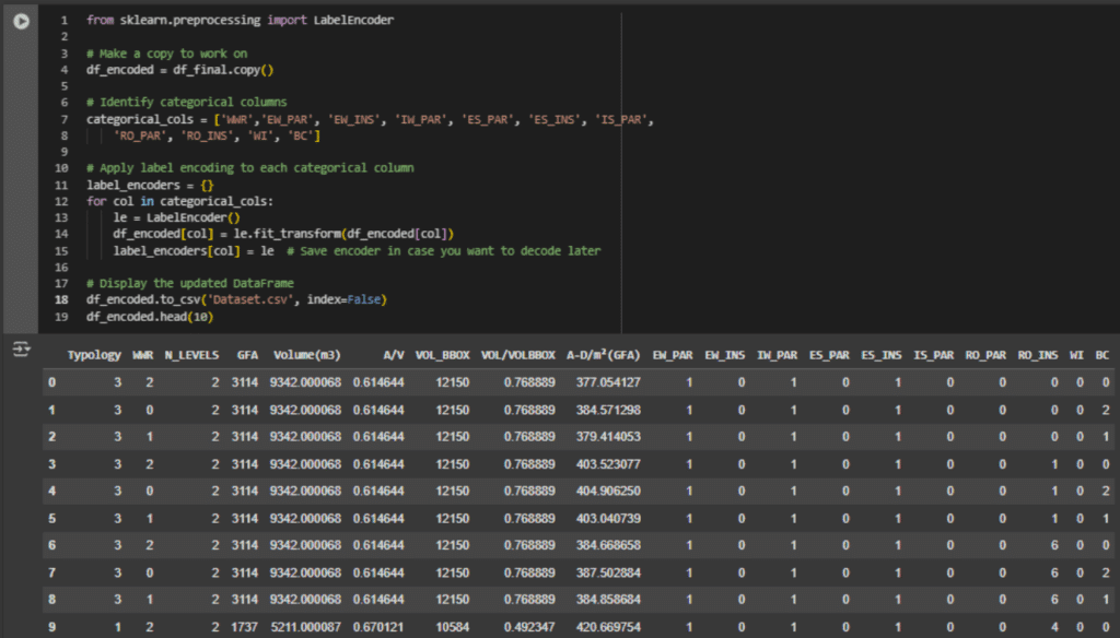
To prepare this dataset for machine learning, categorical variables must be encoded into numerical format. The second image shows the encoding process using Python’s LabelEncoder from the sklearn library. Each material-related column is identified and individually transformed from text labels to integers. This conversion ensures that all features in the dataset are numerical, a requirement for most machine learning algorithms.
The result of this transformation is displayed in the final image, a clean, fully numeric dataset. Categorical values like material types have been replaced by integer codes, making the dataset suitable for model training. This structured, encoded dataset serves as the foundation for developing predictive models that can learn patterns between geometry, materiality, and building performance.
——————————————————————————————————————————————————————————————————————————-
Exploratory Data Analysis
What do we need for training?
That brings us to the Exploratory data analysis. The aim of this section is to reduce dimensionality to the minimum, to limit redundances and unnecessary data and to understand it even more in depth.
_Pairplot_
This pairplot offers an in-depth look at the numerical features of the building performance dataset, revealing key patterns in both their distributions and interrelationships. Each diagonal plot shows the distribution of a variable, while the scatter plots below illustrate how pairs of variables relate to one another.
We observe that GFA and Volume are both strongly right-skewed, indicating that the majority of buildings in the dataset are relatively small, with only a few large outliers. This pattern is also mirrored in the bounding box volume (VOL_BBOX). In contrast, the number of levels (N_LEVELS) displays a multimodal distribution with sharp peaks, likely reflecting standardized floor heights across building types.
The area-to-volume ratio (A/V) is more balanced, with a fairly normal or slightly left-skewed distribution. Meanwhile, VOL/VOLBBOX, a measure of volumetric efficiency, exhibits a bimodal or multimodal distribution. This suggests that buildings in the dataset range from very compact forms to more inefficient or irregular shapes.
Looking at the scatter plots, several strong linear relationships emerge. Notably, GFA and Volume are almost perfectly correlated, as are Volume and VOL_BBOX, a predictable result, since larger buildings occupy more volume and require larger bounding geometries. On the other hand, A/V shows an inverse relationship with Volume, GFA, and VOL_BBOX: as buildings grow in size, their surface-to-volume ratio tends to decrease, which is a common efficiency pattern in architectural design.
Some variables, like VOL/VOLBBOX, show non-linear or less clear trends, with scatter plots revealing clusters or banding patterns. These suggest underlying complexities in shape usage or design logic that might be explored further through clustering or classification techniques.
Overall, the pairplot provides a strong foundation for understanding the geometric structure of the dataset, highlighting patterns that are crucial for both interpretation and predictive modeling.
_Pearson Correlation_
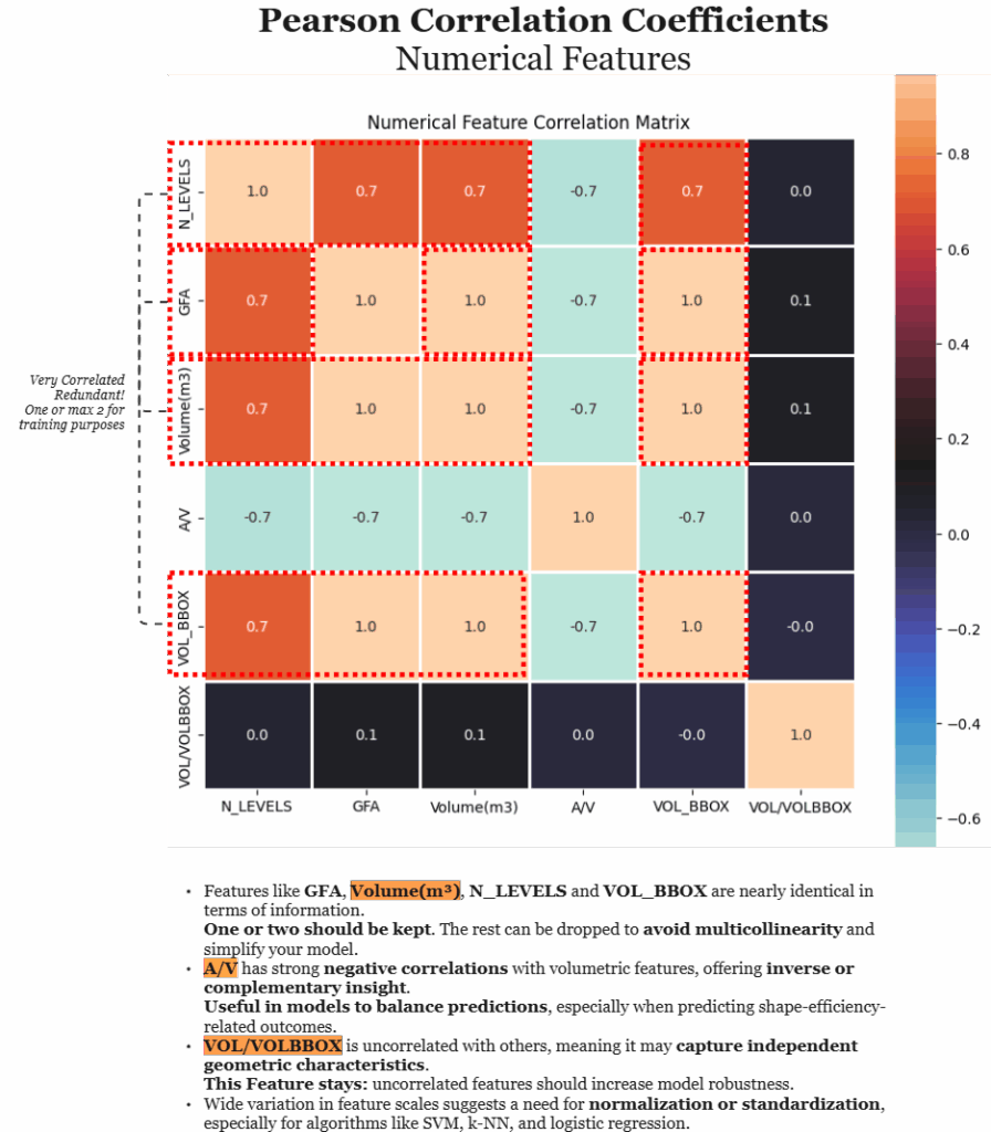
To further understand the relationships between the numerical features in the dataset, a Pearson correlation matrix was generated. This heatmap reveals the strength and direction of linear correlations between each pair of variables, helping to identify redundancy, complementarity, and independent contributions within the data.
Notably, features such as GFA, Volume(m³), N_LEVELS, and VOL_BBOX show very high positive correlations (around 0.7 to 1.0), suggesting they carry nearly identical volumetric information. For modeling purposes, this level of multicollinearity can be problematic, it can inflate variance and reduce interpretability. Therefore, it’s often advisable to retain just one or two of these highly correlated features and drop the rest to simplify the model without significant loss of information.
In contrast, the A/V (area-to-volume) ratio shows strong negative correlations with the volumetric features. This inverse relationship is geometrically intuitive, larger, more compact buildings tend to have lower surface-area-to-volume ratios. This makes A/V a valuable complementary feature, particularly in models concerned with shape-efficiency or energy-related outcomes.
The standout feature in this matrix is VOL/VOLBBOX, which shows almost no correlation with any other variable. This suggests it may represent a distinct geometric property, perhaps shape irregularity or inefficiency, not captured by the other features. Including such independent features can improve model robustness and enhance the range of captured patterns.
Lastly, the wide range of correlation values and feature scales underscores the importance of normalization or standardization prior to model training, especially for algorithms sensitive to feature magnitude, such as SVMs or logistic regression.
Overall, this correlation matrix helps inform feature selection strategies, encouraging a balance between removing redundancy and preserving meaningful, diverse predictors for robust machine learning models.
_Principal Component Analysis_
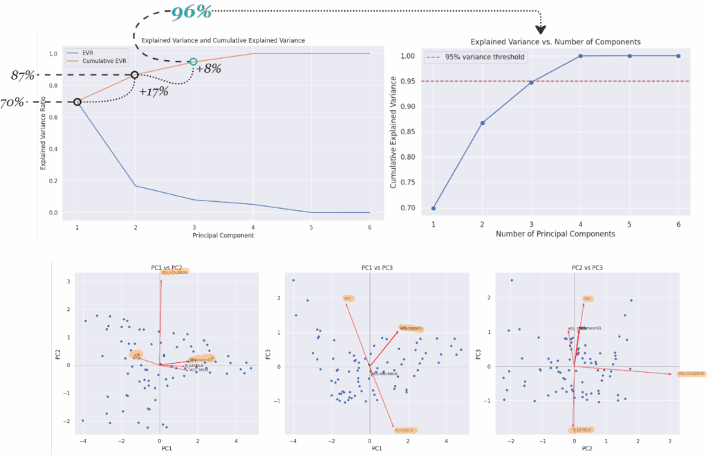
To reduce dimensionality while preserving the most meaningful information, a Principal Component Analysis (PCA) was conducted on the numerical features of the dataset. The top graphs illustrate the explained variance ratio (EVR) and the cumulative explained variance for each principal component (PC). The first two components alone account for approximately 87% of the total variance, with the third component pushing this to 96%, exceeding the common 95% threshold used for dimensionality reduction. This means that with just three components, we can retain nearly all of the dataset’s original information.
The bottom row of scatter plots visualizes how these principal components relate to the original variables. These biplots show the direction and strength of feature contributions (red vectors) across combinations of principal components.
- In the PC1 vs PC2 plot, we see that
VOL/VOLBBOXis the most distinct contributor to PC2, indicating it captures shape efficiency orthogonal to size-based attributes. - PC1 vs PC3 highlights
A/Vas a strong contributor to PC3, suggesting it holds complementary shape-efficiency information, independent of total volume. - PC2 vs PC3 shows
N_LEVELSandVOL/VOLBBOXpushing in opposite directions, reinforcing the idea that PCA reveals contrasting geometric dimensions, compactness versus stacking.
Together, these plots confirm that while features like GFA, volume, and bounding box volume overlap in information, shape-efficiency metrics like A/V and VOL/VOLBBOX capture independent, valuable dimensions. PCA not only streamlines the dataset for modeling but also helps interpret the underlying geometric structure by clustering related features and highlighting unique ones.
——————————————————————————————————————————————————————————————————————————-
ML-Approach
Which algorithm is the best fit?
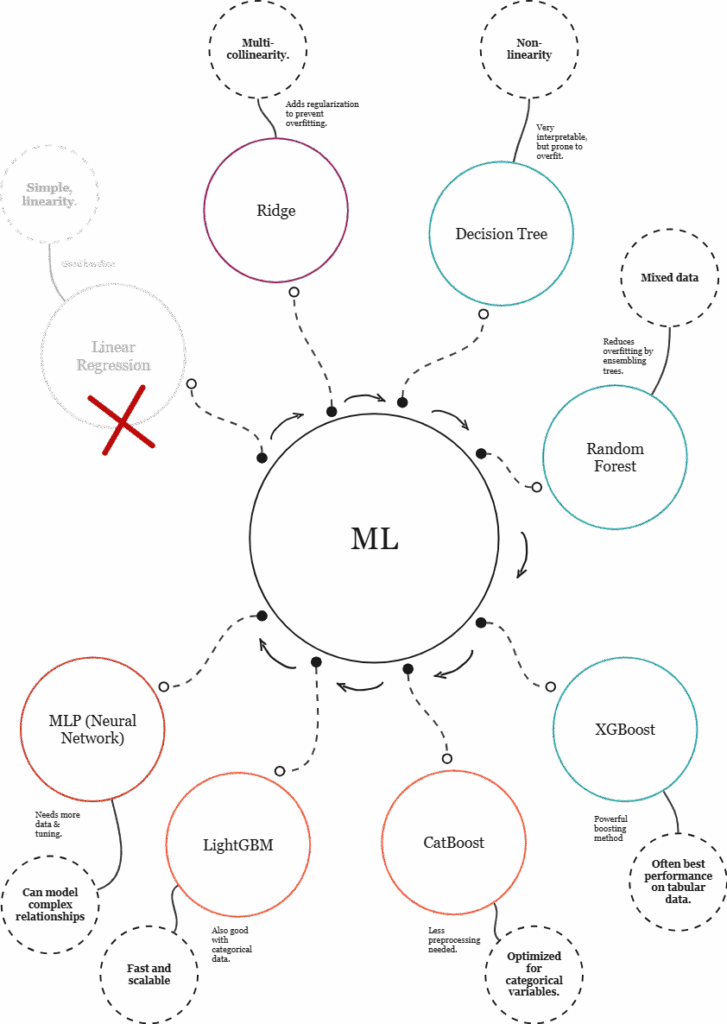
To identify the most suitable machine learning model for the building performance prediction task, a strategic and iterative approach is essential, beginning with simple models and progressing toward more advanced techniques as needed.
The process typically starts with linear regression, a straightforward model that provides a performance baseline. While it’s useful for initial comparisons, it assumes linear relationships among features, a limitation in this case, given the presence of non-linear patterns and multicollinearity between variables such as GFA, Volume, and bounding box dimensions. As such, linear regression is quickly ruled out as insufficient for capturing the complexity of the dataset.
To address multicollinearity while remaining within the linear modeling family, Ridge regression with polynomial features introduces regularization to stabilize coefficients. Although it offers a more robust alternative to linear regression, Ridge is still bound by linear assumptions and may struggle to model the complex geometric relationships present in the data.
The next step is to move toward models that can capture non-linear relationships. Decision trees are well-suited for this, offering interpretable rules and the ability to work with both numerical and categorical variables. However, their high variance makes them prone to overfitting. This is mitigated by random forests, which aggregate many trees to improve generalization. Random forests strike a good balance between accuracy, robustness, and interpretability, making them a strong candidate for this type of structured, tabular data.
For more advanced modeling, boosting algorithms like XGBoost, LightGBM, and CatBoost are excellent options. These models build trees sequentially, each correcting the errors of its predecessor. XGBoost is known for high performance and flexibility, especially with complex, non-linear datasets. LightGBM is particularly efficient on large datasets and handles categorical features effectively. CatBoost stands out for its native support of categorical variables, reducing the need for extensive preprocessing and making it especially well-suited for mixed datasets like this one.
Lastly, multilayer perceptrons (MLPs) or neural networks can be considered for modeling more abstract or intricate patterns. While powerful, they typically require more data, greater tuning, and longer training times, and may not outperform tree-based models on structured tabular data unless additional data types (e.g., temporal or image data) are introduced.
In summary, the recommended path begins with Ridge regression for a regularized baseline, followed by random forest for a strong general-purpose model. From there, CatBoost and XGBoost are the most promising candidates for high performance. MLPs may be explored later for experimentation or hybrid models. This layered strategy ensures both interpretability and performance are optimized throughout the model selection process.
_ML-Parametric Approach_
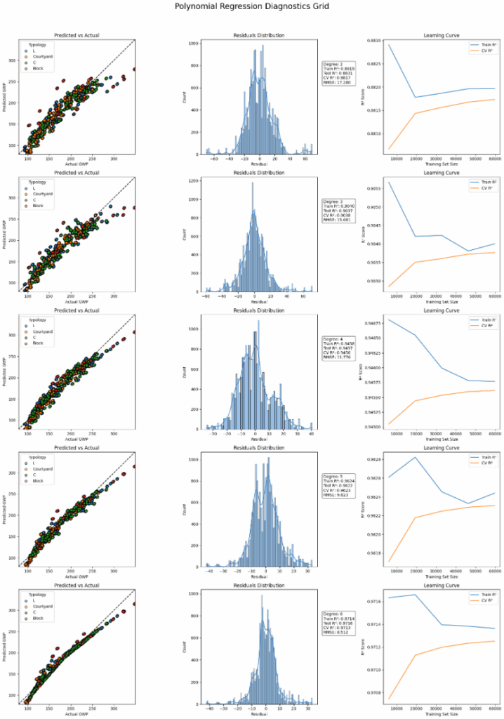
Our baseline starts with the evaluation different degrees of polynomiality we can see a boost in performance up to the degree of 5. Nevertheless our benchmarks are not completely fulfilled.
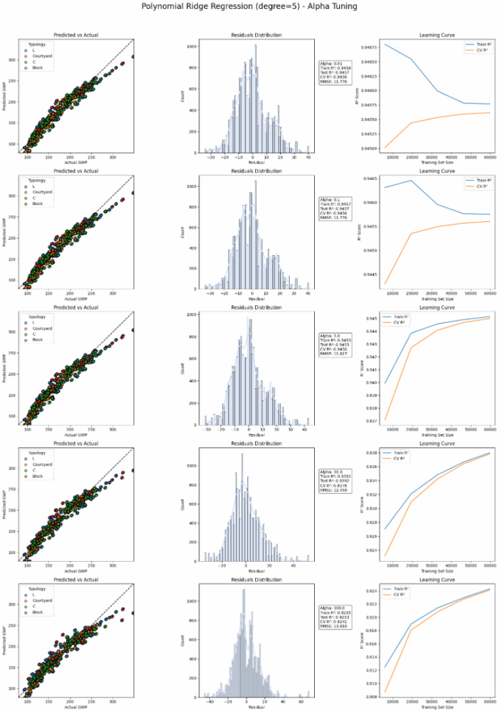
We took the polynomial base of 5 from the previous example and regularized l2 with Ridge. Varying alpha improves the learning curve but still does not take us to the goal.
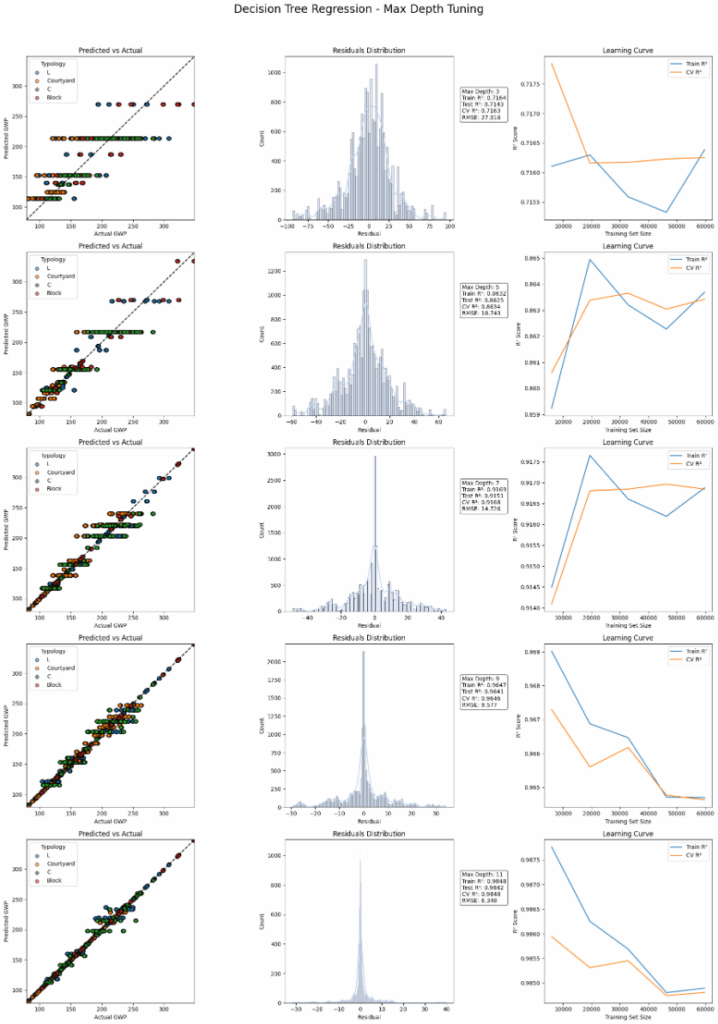
Next we explore how decision trees perform on different depths. We see that all numerical metrics are fulfilled, nevertheless the diagrams show visually signs of overfitting in all of them.
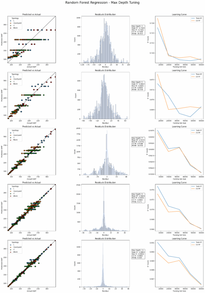
Exploring Random Forests gave us unfortunately the same results as decision trees. The number of estimators was kept low at 30. Perhaps increasing it to higher values would bring more stability, of course as well with increased computation power.
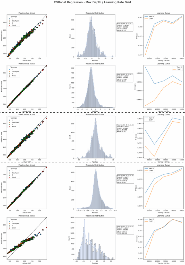
The breakthrough comes once XGBoost appears. At a depth o 5 and a learning rate of 0.05 the results look promising. This is our first candidate for deployment.
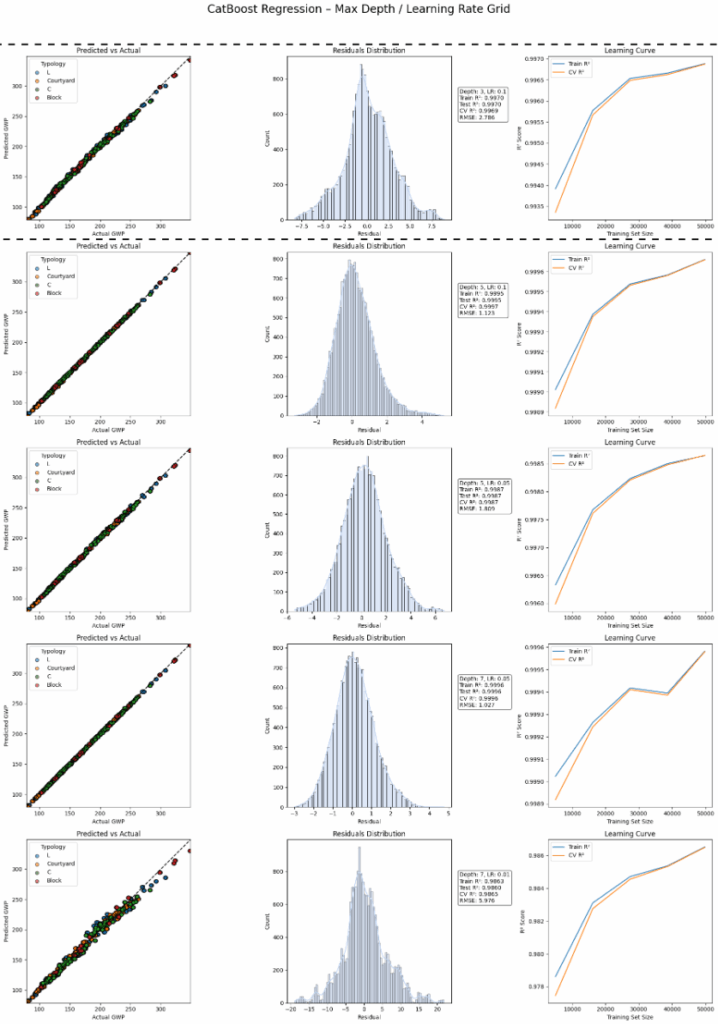
As we have many categorical features, we tested as well CatBoost. The high performance of this model is obvious. We get our second candidate from this batch with a depth of 3 and a learning rate of 0.1.
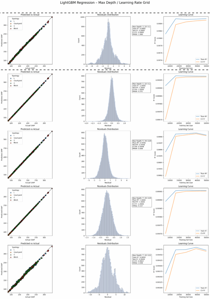
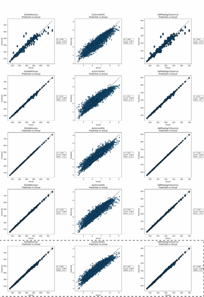
LightGBM at depth 3 generalizes well while maintaining speed. It’s slightly less accurate than XGBoost or Catboost but the training process is faster.
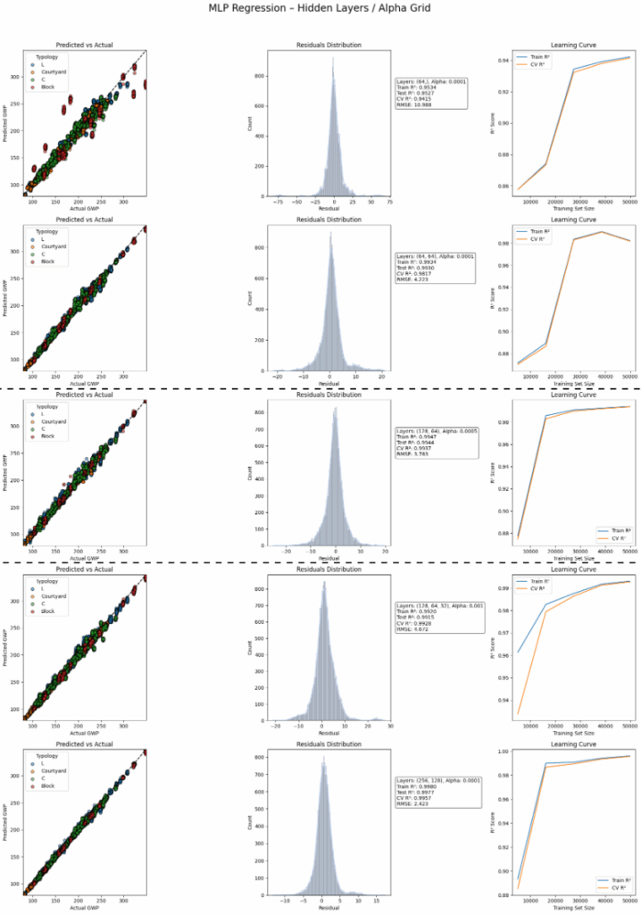
MLP with two hidden layers balances flexibility and stability. While there’s some variance, this setup avoids both severe underfitting and catastrophic overfitting.
In the pursuit of training a model for multiple outputs we explored further the use of MLPs. The best MLP model from the previous step shows high prediction accuracy for key metrics like GWPtot and Operational Carbon. However, performance drops on outputs like C2 and D stages, suggesting the need for model refinement or separate models for some targets.
——————————————————————————————————————————————————————————————————————————-
SHapley Additive exPlanations
How to double check the model selection?
We decided to move on with the selected models into deployment. Our favorite is, nevertheless, lightGBM due to its fast training and high performance. So we will analyze it further with SHAP.
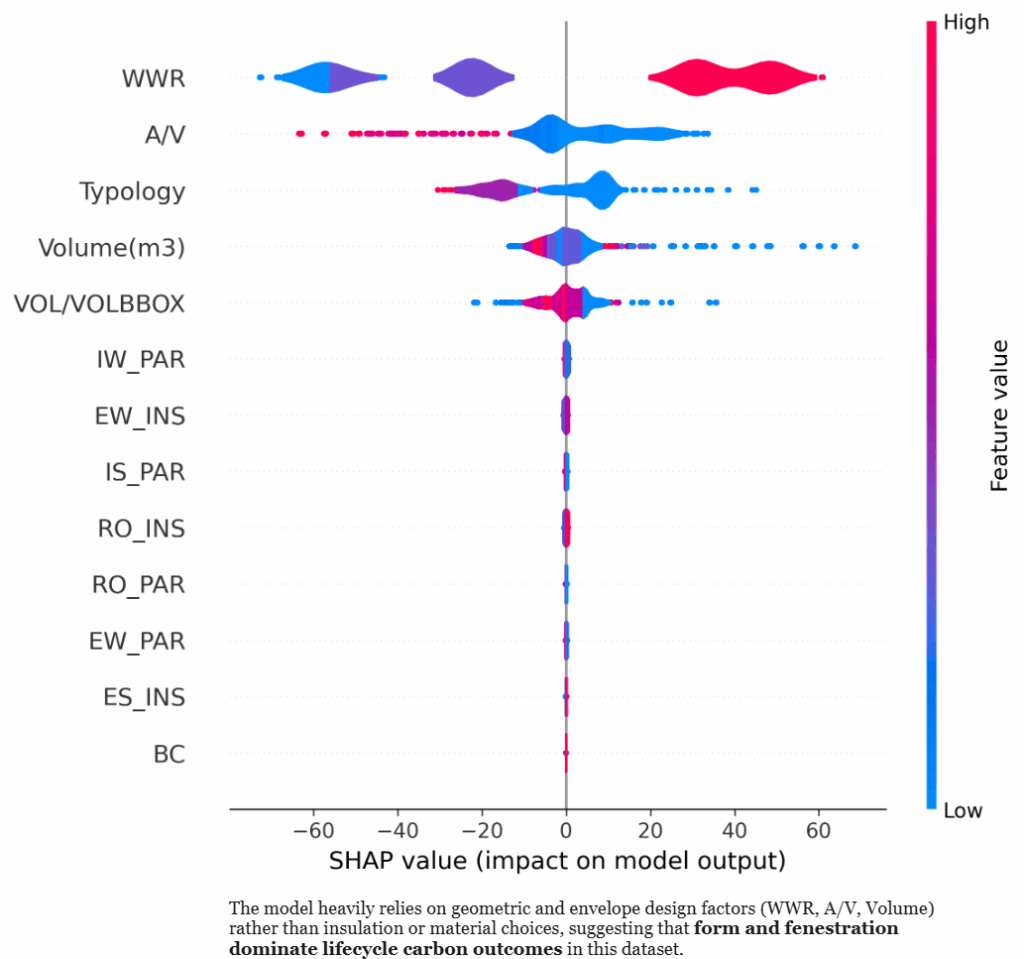
This violin summary plot ranks features by importance. We see that WWR and A/V ratio have the largest impact, positive or negative, on the predicted GWP, with clear directional trends across their ranges.
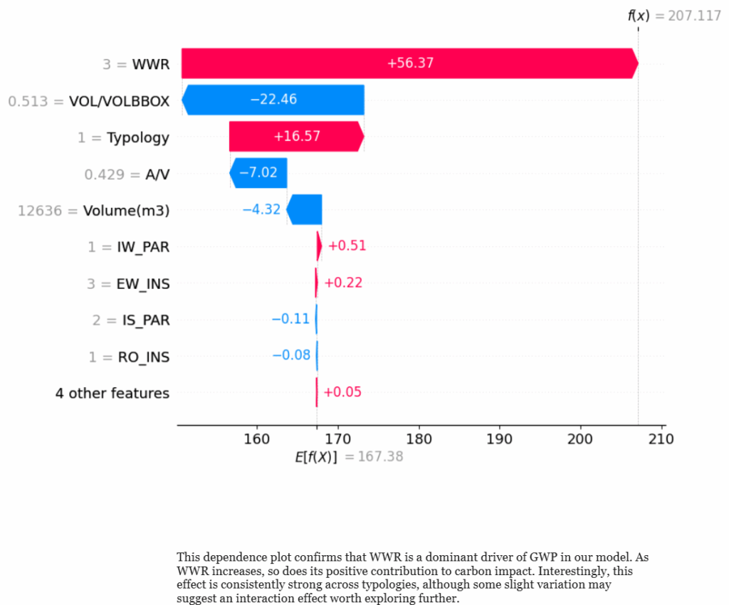
This waterfall plot explains one individual prediction. It starts from the base value and shows how each feature pushes the prediction up or down. WWR increases the GWP significantly, while VOL/VOLBBOX reduces it, making it a key design driver
——————————————————————————————————————————————————————————————————————————-
Deployment
How to test the model in a real world workflow?
We integrated the top tier models into a grasshopper driven workflow. This allows us to get real time feedback about the GWP of our design via the predictions of the different models.
Integration in GH
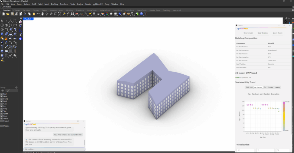
Surrogate Models
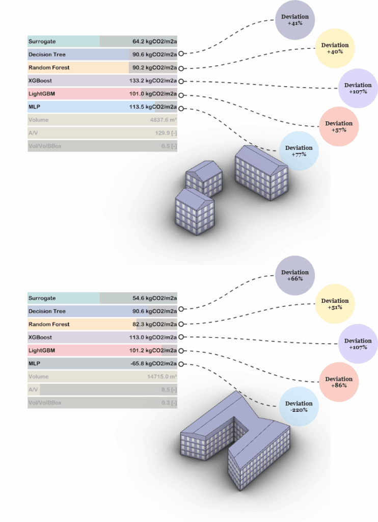
To further evaluate the machine learning models, two test cases were developed using surrogate models, simplified simulations that estimate environmental impact based on a reduced set of inputs. These surrogates serve as lightweight benchmarks against which we can compare the ML model predictions.
The results reveal an interesting insight: the models with the highest predictive accuracy during training and validation, such as XGBoost, LightGBM, and MLP, show the largest deviations from the surrogate models in both test cases. For instance, in the smaller multi-volume building (top image), XGBoost overshoots the surrogate estimate by over 100%, while MLP predicts a deviation of +77%. Similarly, in the larger L-shaped building (bottom image), MLP even predicts a negative value, deviating by -220%.
At first glance, these deviations might suggest poor performance. However, the key takeaway is that this does not imply the models are incorrect. On the contrary, it likely means that the machine learning models are responding to more nuanced and detailed features from the full dataset, features that the surrogate models do not capture. In contrast, models like Decision Tree or Random Forest, which perform more conservatively, align more closely with the surrogate, showing lower deviations but potentially less sensitivity to geometric and material complexity.
This comparison underscores a fundamental point: simplified surrogates are useful for benchmarking, but high-performing models will inevitably diverge when the underlying data captures a richer set of conditions. The deviation, in this context, reflects model depth and detail, not necessarily inaccuracy.
——————————————————————————————————————————————————————————————————————————-
Conclusion
This study conducted a comprehensive comparison of various regression models, ranging from interpretable polynomial approaches to powerful ensemble methods like XGBoost, LightGBM, CatBoost, and neural networks
The goal was the identification of most suitable models for real-time GWP (Global Warming Potential) prediction in architectural applications.
Through rigorous evaluation of prediction accuracy, generalization capacity, computational efficiency, and explainability via SHAP analysis, we found that LightGBM offers the best balance. It delivers high accuracy with controlled overfitting and fast inference, making it well-suited for integration into a real-time Grasshopper-based application.
The outcome is not only a robust prediction model but also a transparent, interactive workflow that enables designers and decision-makers to estimate the environmental impact of their designs with immediate feedback, empowering more sustainable choices from the earliest design stages.
——————————————————————————————————————————————————————————————————————————-
Next Steps
The work is far from being done…
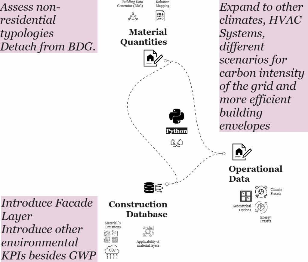
This diagram outlines future directions to enhance the current data-driven framework for building performance assessment, with a focus on expanding its scope, improving environmental depth, and increasing flexibility.
One key development is the call to assess non-residential typologies and detach the workflow from the Building Data Generator (BDG). By decoupling from the BDG and introducing new building types, such as offices, schools, or commercial spaces, the system can move beyond its current residential focus, making it more broadly applicable across the built environment.
Equally important is the proposal to expand the operational analysis to include a wider range of climates, HVAC systems, and energy scenarios. This would enable the model to account for regional variations, simulate future grid conditions, and assess the impact of more efficient building envelopes under different environmental contexts. Such flexibility would support robust scenario planning and enhance the model’s usefulness for climate-responsive design.
In parallel, there is an opportunity to deepen the environmental modeling by introducing facade layers and additional sustainability indicators beyond Global Warming Potential (GWP). Metrics such as embodied energy, water usage, and material circularity could provide a more comprehensive view of environmental impact, aligning the tool with broader life-cycle thinking.
Finally, strengthening the construction database, by enriching material emissions data and refining the applicability of material layers, would improve the accuracy and realism of both material quantity estimations and lifecycle assessments. This would better ground the model in construction practice and regional material standards.
Together, these proposed enhancements chart a clear path forward: making the framework more inclusive, scalable, and aligned with both environmental goals and real-world complexity.