
Predicting Building Energy Performance: A Machine Learning Approach to Energy Use Intensity (EUI)
- Introduction: Understanding Energy Use Intensity (EUI)
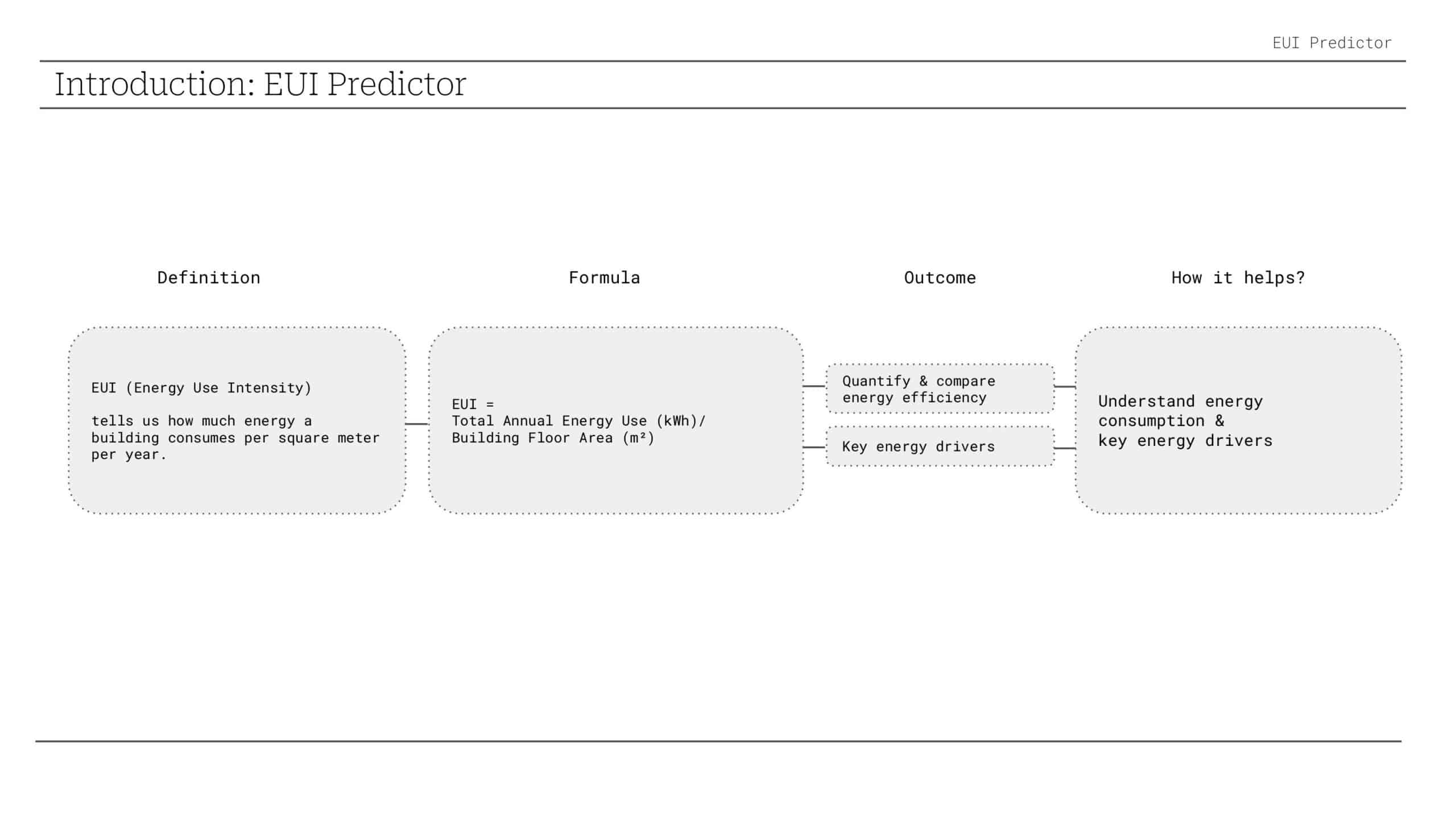
In the world of sustainable architecture and building design, understanding energy consumption is crucial for creating efficient, environmentally responsible structures. Energy Use Intensity (EUI) serves as a fundamental metric that tells us how much energy a building consumes per square meter per year.
EUI Formula:
EUI = Total Annual Energy Use (kWh) / Building Floor Area (m²)
This metric helps us:
- Quantify & Compare energy efficiency across different buildings
- Understand Energy Consumption patterns and identify key energy drivers
- Make Data-Driven Decisions in the design process
2. Project Overview: The EUI Predictor
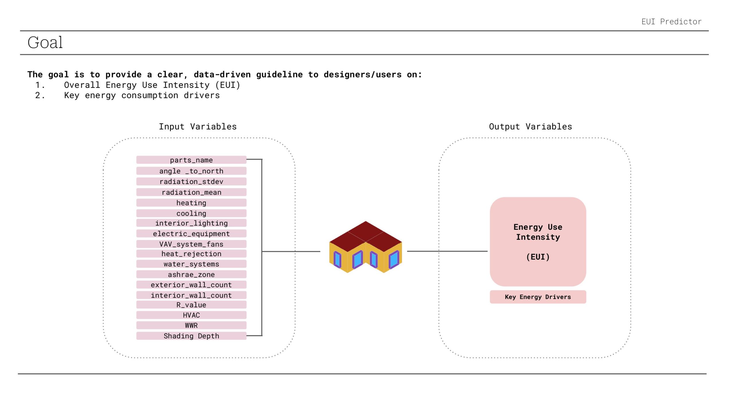
Our EUI Predictor project aims to provide clear, data-driven guidelines to designers and users by predicting:
- Overall Energy Use Intensity (EUI)
- Key energy consumption drivers
The system takes various input variables related to building geometry, systems, and environmental conditions to predict energy performance outcomes.
Input Variables Include:
- Building geometry (parts_name, angle_to_north)
- Environmental factors (radiation_stdev, radiation_mean)
- HVAC systems and energy loads (heating, cooling, VAV_system_fans)
- Building envelope characteristics (WWR, R_value, shading_depth)
- Climate data (ashrae_zone)
3. Methodology: From Individual Units to Building-Scale Analysis
Individual- scale to building scale analysis
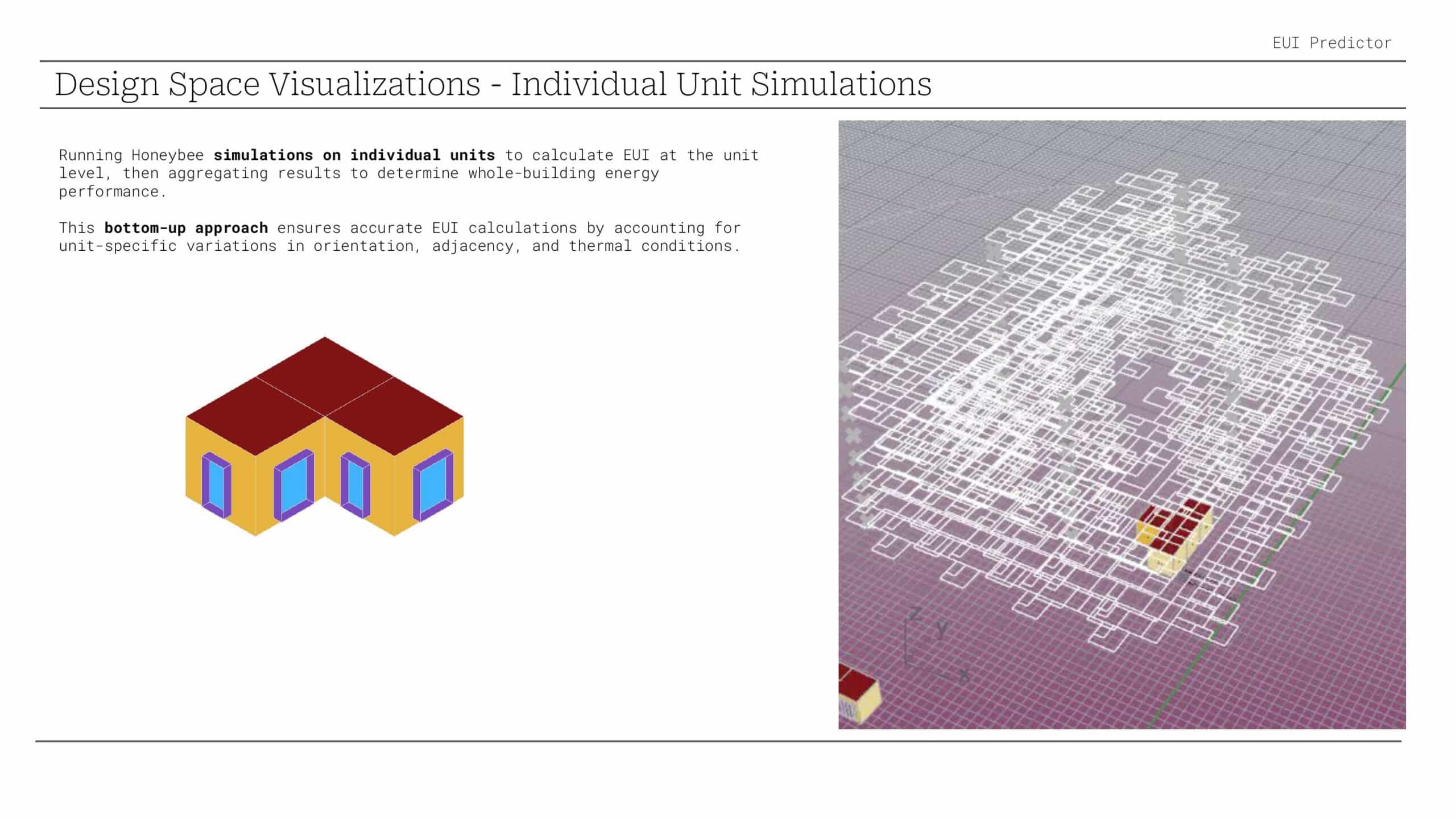
Our approach begins with a bottom-up methodology, running Honeybee simulations on individual building units to calculate EUI at the unit level. We then aggregate these results to determine whole-building energy performance.
This approach ensures accurate EUI calculations by accounting for:
Unit-specific variations in orientation
Adjacency effects between units
Thermal condition differences throughout the building
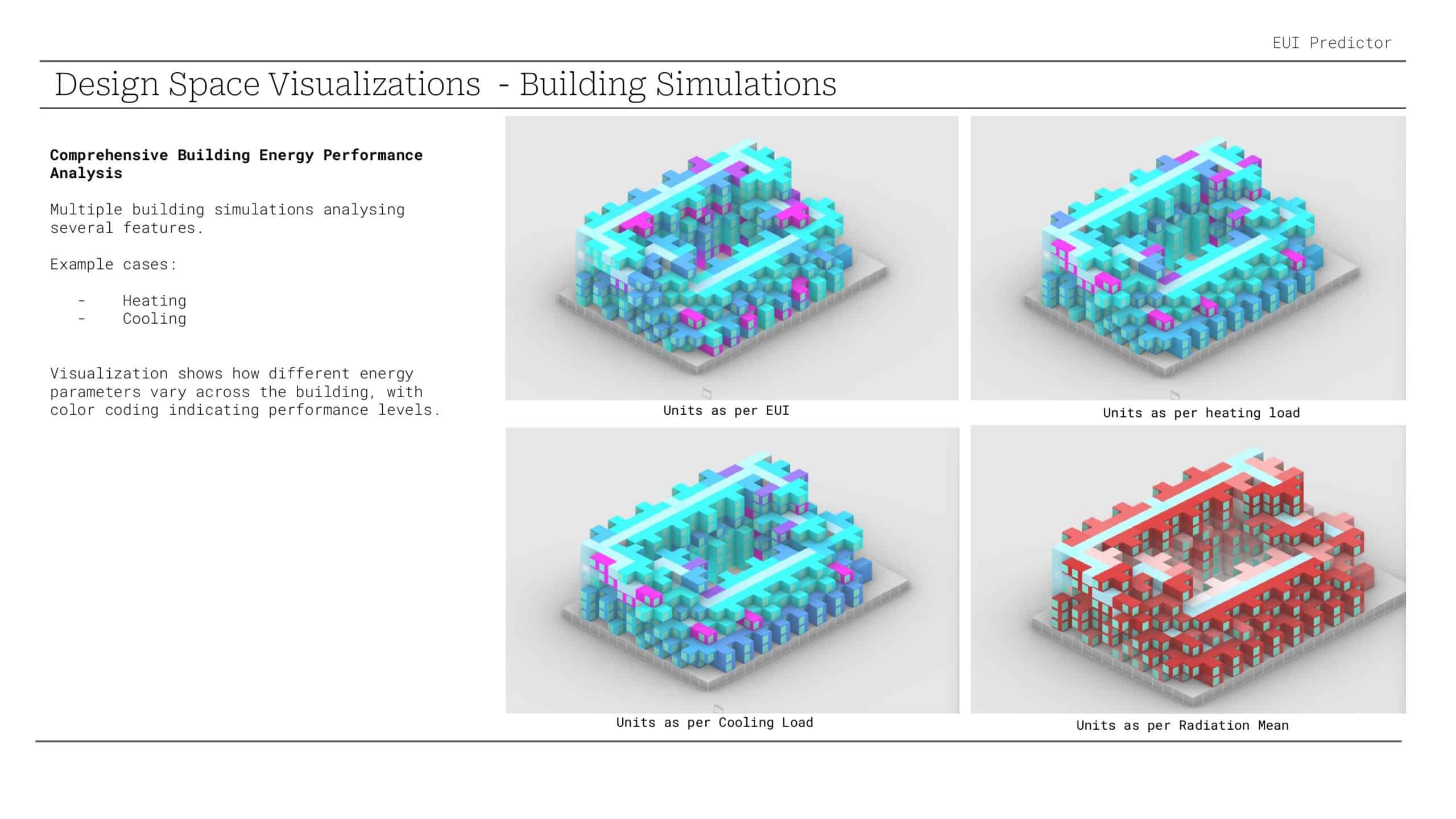
Building-Scale Comprehensive Analysis
Moving beyond individual units, we conducted comprehensive building energy performance analysis across multiple parameters:
- Heating Load Distribution – Understanding thermal requirements
- Cooling Load Patterns – Analyzing climate control needs
- EUI Variations – Mapping energy intensity across units
- Solar Radiation Impact – Evaluating environmental factors
Our visualizations use color coding to indicate performance levels, making it easy to identify high and low-performing areas within the building.
4. Dataset Analysis: Understanding Our Data
Dataset Composition
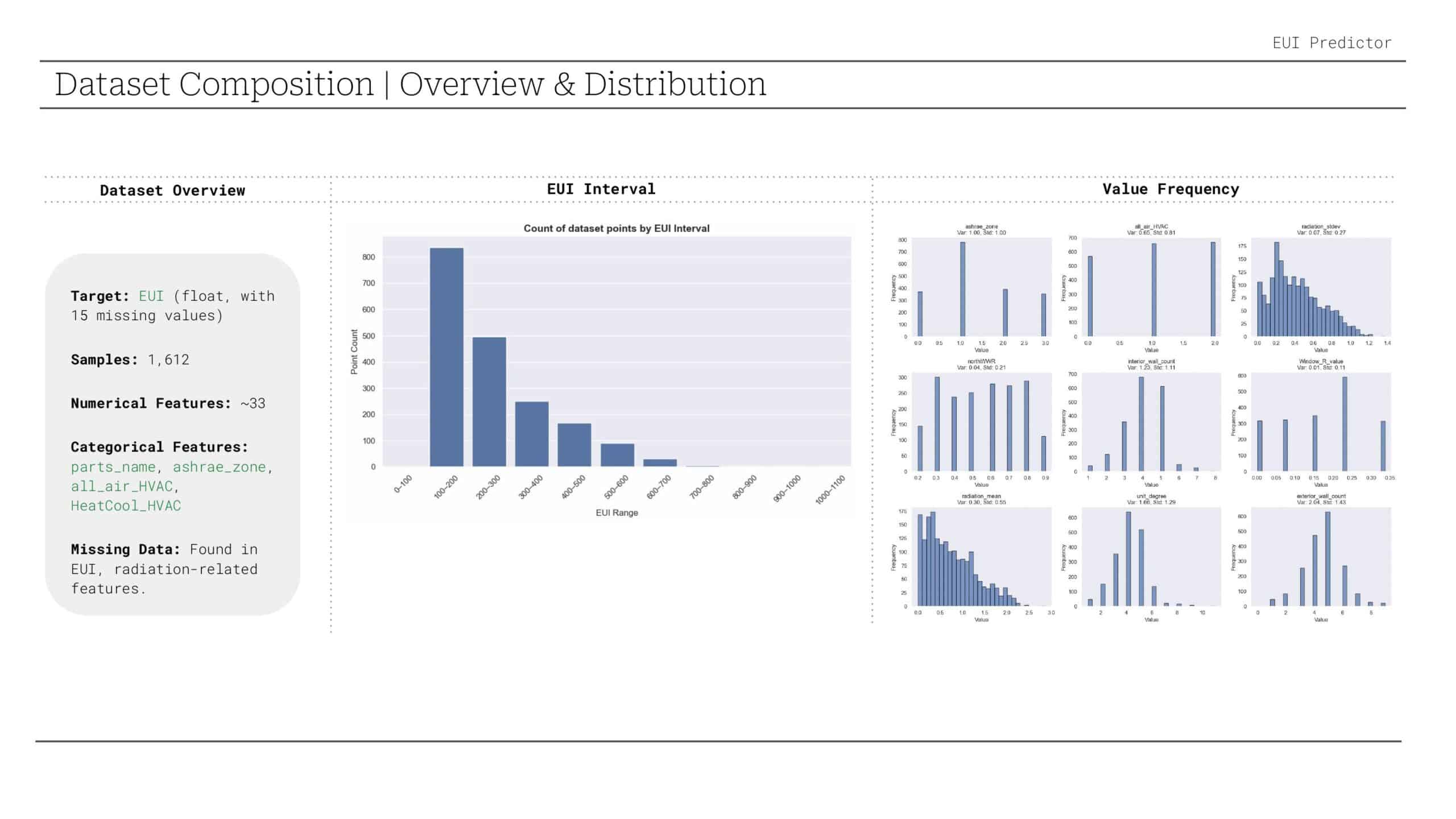
Our comprehensive dataset includes:
- Total Samples: 1,612 building units
- Target Variable: EUI (float, with 15 missing values)
- Numerical Features: ~33 continuous variables
- Categorical Features: parts_name, ashrae_zone, HVAC system types
- Data Quality: Missing data found primarily in EUI and radiation-related features
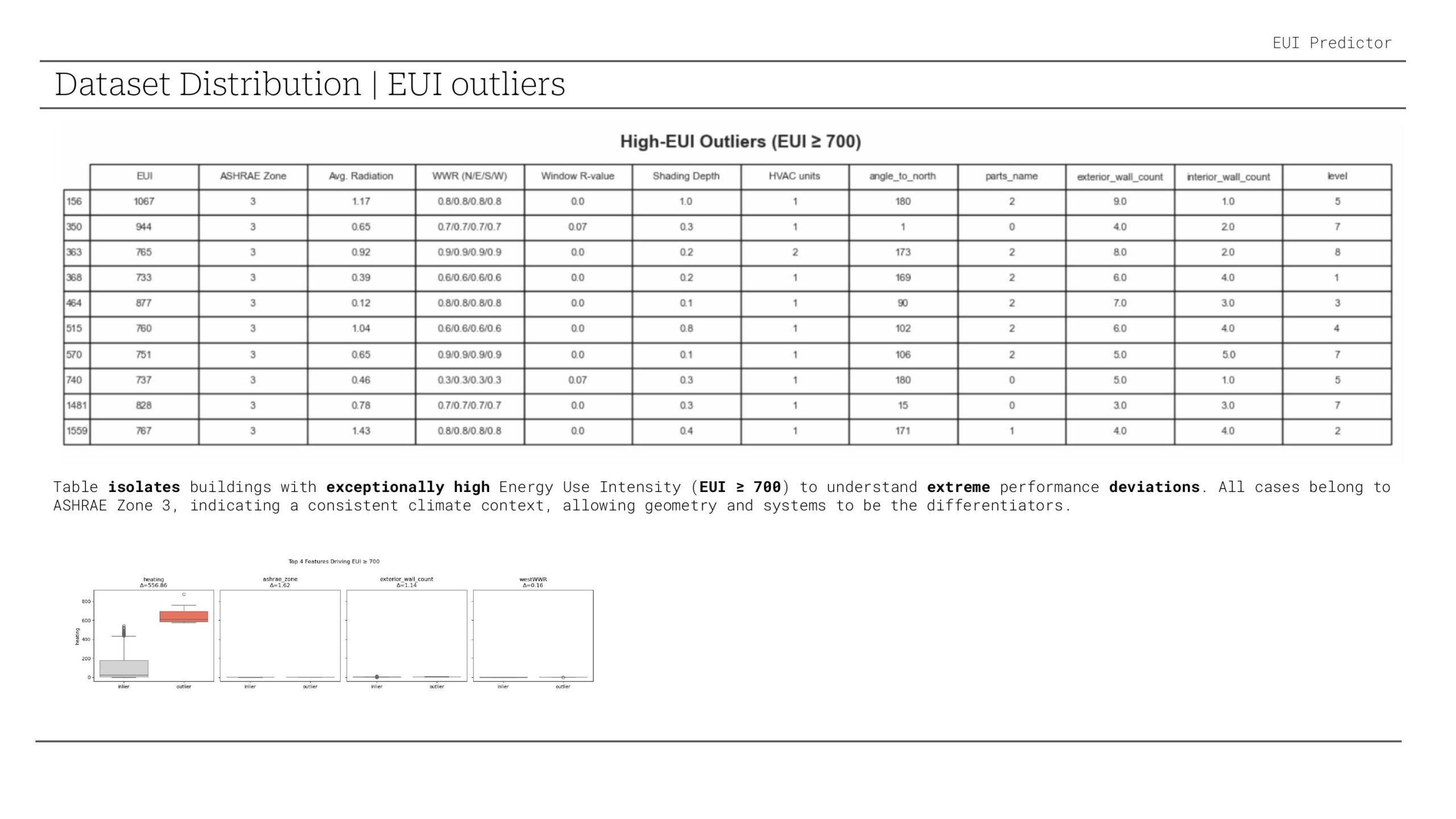
5. Identifying Performance Outliers
A critical part of our analysis involved identifying buildings with exceptionally high Energy Use Intensity (EUI ≥ 700). Interestingly, all extreme cases belonged to ASHRAE Zone 3, indicating consistent climate context. This finding suggests that geometry and system configurations are the primary differentiators in extreme performance cases.
6. Feature Engineering: Extracting Meaningful Patterns
Principal Component Analysis (PCA)
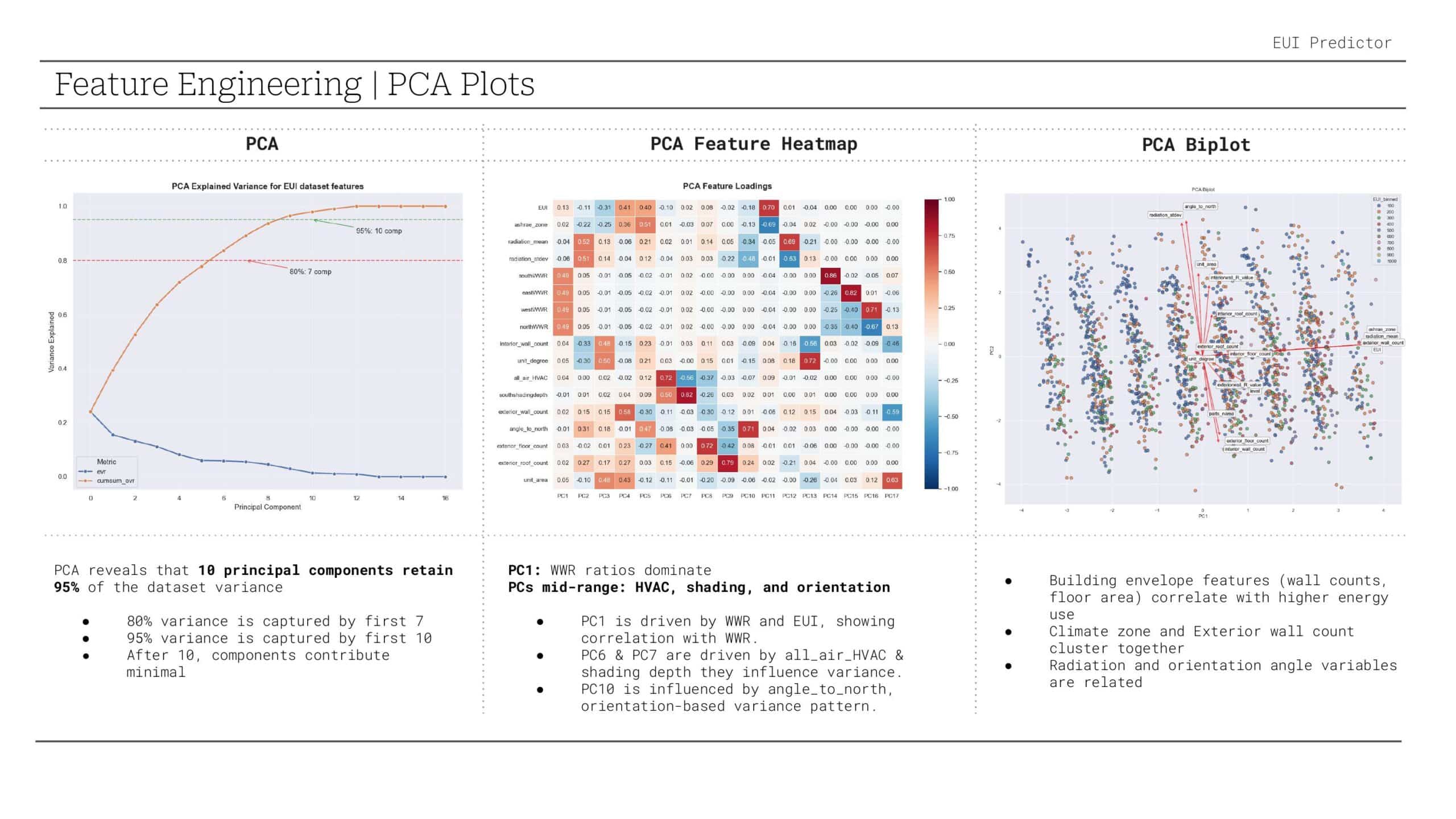
Our PCA analysis revealed crucial insights about data structure:
- 95% of dataset variance is retained with just 10 principal components
- 80% variance captured by the first 7 components
- Key finding: Building envelope features (wall counts, floor area) correlate strongly with higher energy use
Component Analysis:
- PC1: Dominated by Window-to-Wall Ratio (WWR) and EUI correlation
- PC6 & PC7: Influenced by HVAC systems and shading depth
- PC10: Driven by building orientation (angle_to_north)
7. Advanced Visualization Techniques
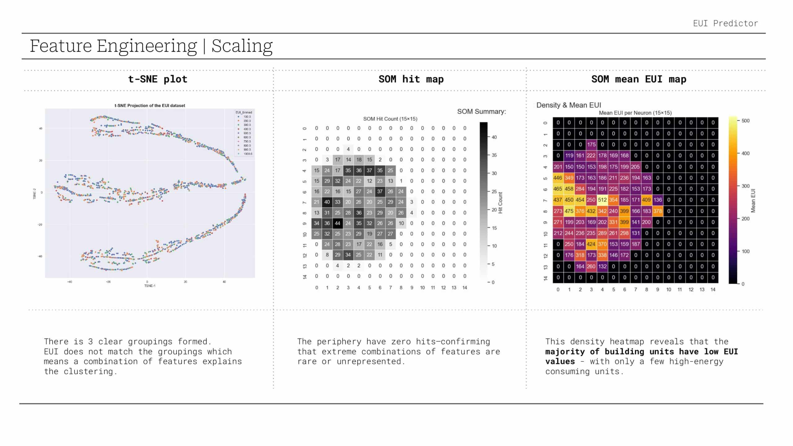
We employed multiple visualization techniques to understand data clustering:
- t-SNE plots revealed three clear groupings in the data
- Self-Organizing Maps (SOM) confirmed that extreme feature combinations are rare
- Density heatmaps showed that most building units have low EUI values, with only a few high-energy consuming outliers
Feature Importance Analysis
Using Random Forest analysis, we identified the most critical predictors:
- ashrae_zone – The dominant predictor (climate zone)
- all_air_HVAC – HVAC system type
- Window_R_value – Thermal resistance of windows
This ranking highlighted the overwhelming importance of climate zone classification in energy prediction.
8. Machine Learning Model Development
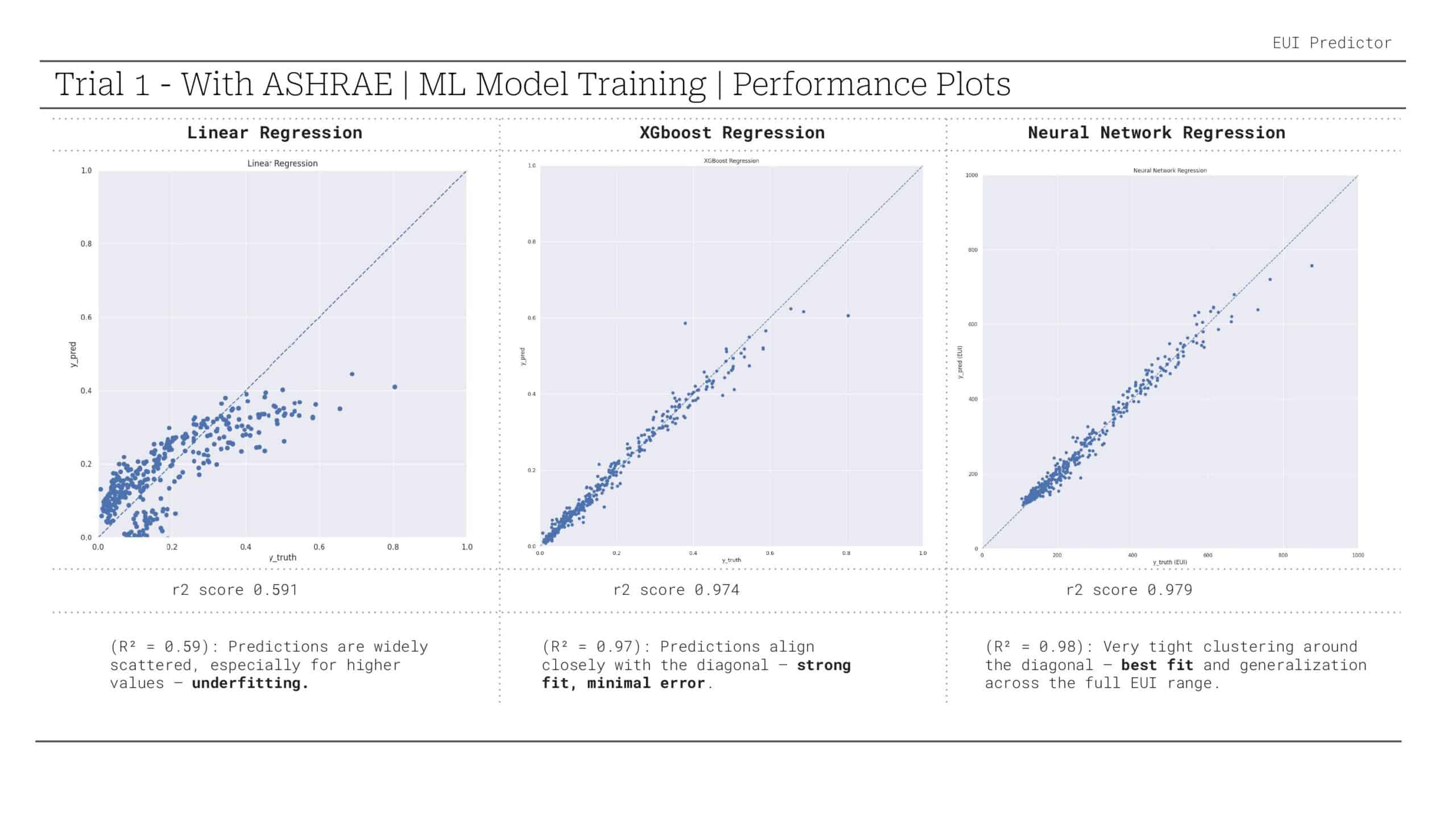
Trial 1: Including ASHRAE Zone
Our first trial included all features, particularly the ASHRAE zone classification:
Results:
- Linear Regression: R² = 0.591 (significant underfitting)
- XGBoost Regression: R² = 0.974 (strong performance)
- Neural Network: R² = 0.979 (best performance)
9. Neural Network Training Analysis
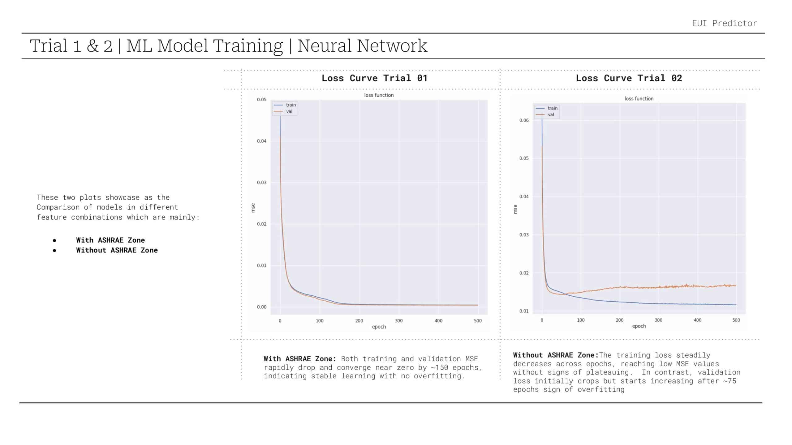
Comparing loss curves between trials:
Trial 1 (With ASHRAE): Both training and validation MSE rapidly converged near zero by ~150 epochs, indicating stable learning without overfitting.
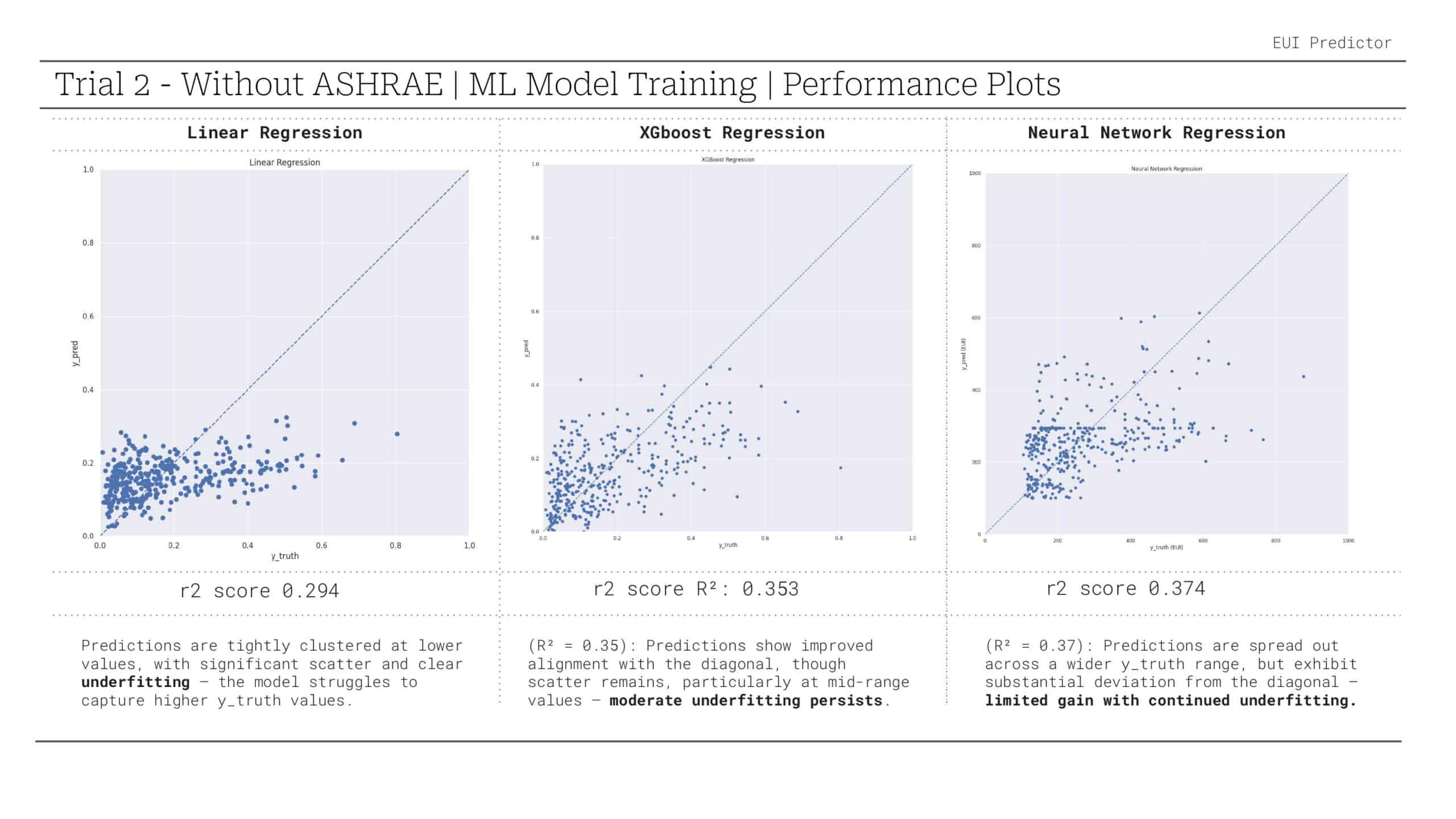
Trial 2 (Without ASHRAE): Training loss decreased steadily, but validation loss began increasing after ~75 epochs, showing clear signs of overfitting.
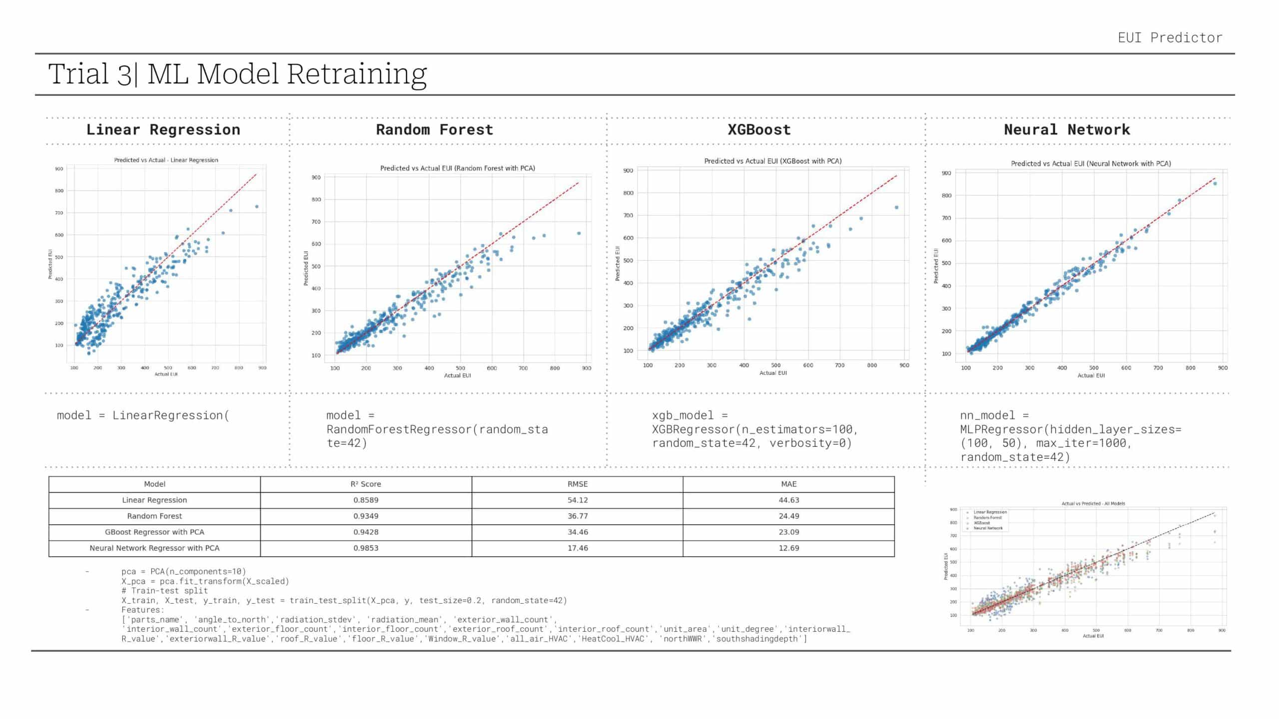
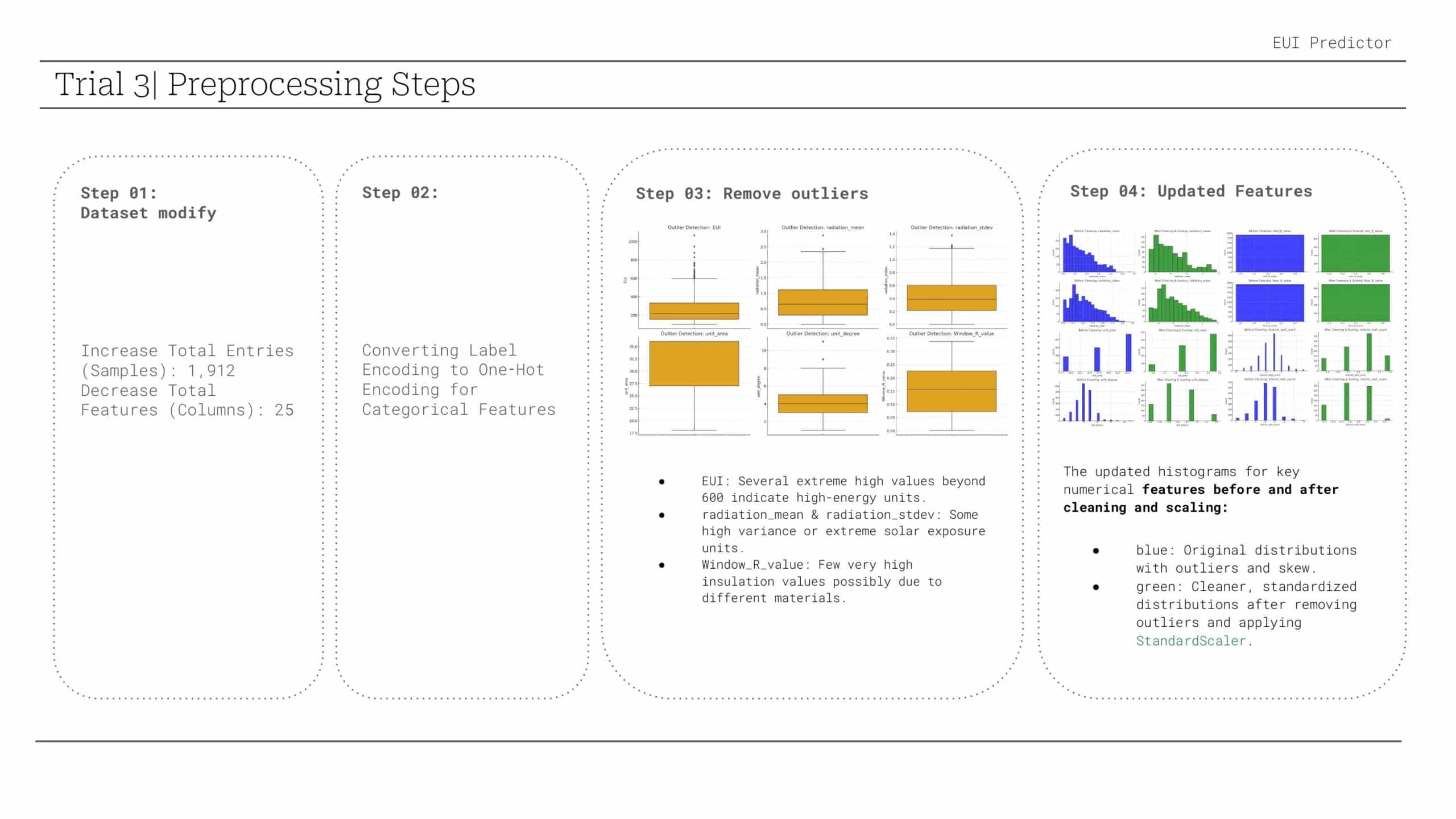
10. Model Optimization: Trial 3
Advanced Preprocessing Pipeline
For our final trial, we implemented a comprehensive preprocessing approach:
Step 1: Dataset expansion to 1,912 samples with 25 refined features Step 2: One-hot encoding for categorical variables
Step 3: Outlier removal targeting extreme values in EUI, radiation metrics, and Window_R_value Step 4: Feature standardization using StandardScaler
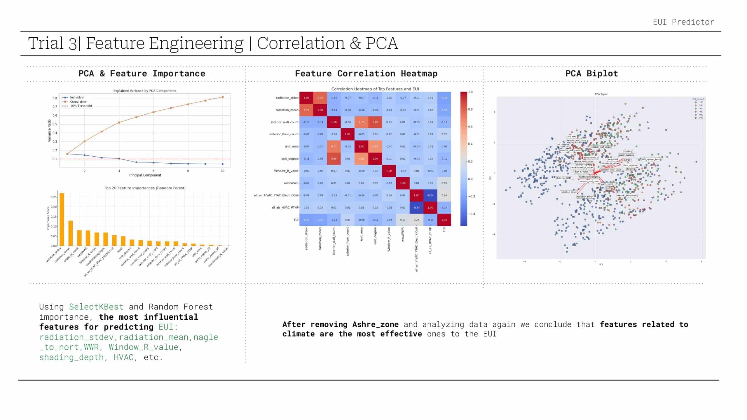
Refined Feature Analysis
After removing ASHRAE zone and re-analyzing, we identified climate-related features as most effective:
- radiation_stdev, radiation_mean
- angle_to_north
- WWR, Window_R_value
- shading_depth, HVAC systems
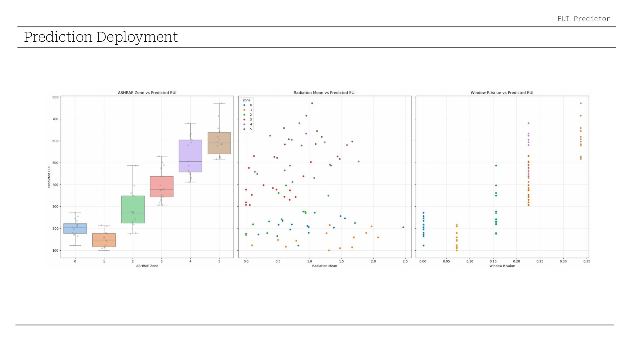
11. Deployment and Practical Application
Real-World Implementation
Our EUI Predictor has been deployed for practical use, allowing designers to:
- Input building parameters through an intuitive interface
- Receive instant EUI predictions
- Compare predicted vs. simulated values
- Identify optimization opportunities
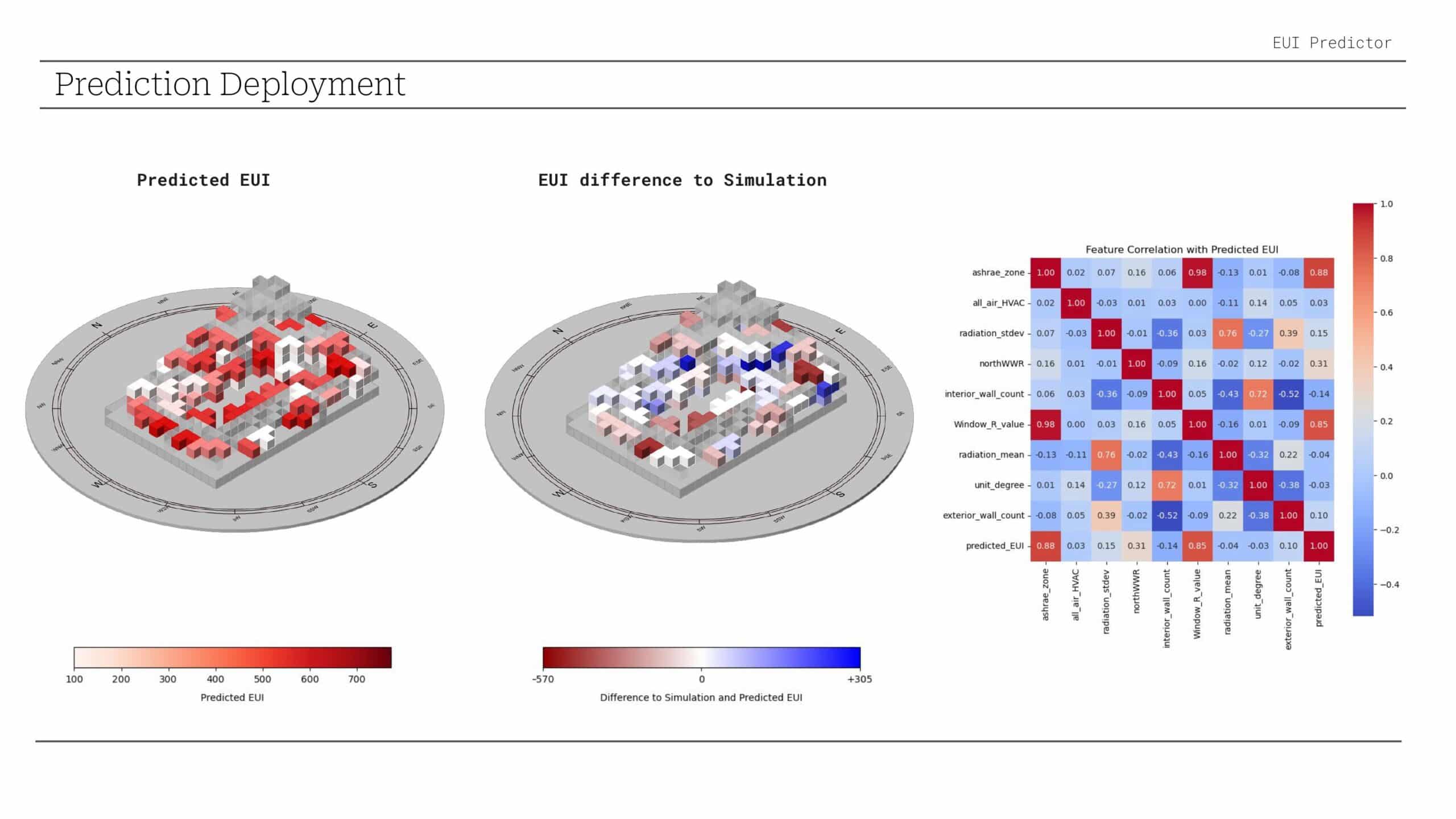
The deployment interface shows both predicted EUI values and differences compared to detailed simulation results, enabling users to understand prediction accuracy and make informed design decisions.
12. Deployment and Practical Application
13. Key Findings and Critical Insights
Major Discoveries
- Climate Zone Dominance: ASHRAE zone classification proved to be the overwhelmingly dominant factor in EUI prediction, highlighting the critical importance of climate in building energy performance.
- Model Dependency Risk: Removing the ASHRAE zone led to dramatic performance degradation, revealing dangerous over-reliance on a single variable.
- Feature Interaction Complexity: The model struggled to learn meaningful patterns from geometric and system features when climate data was absent.
14. Conclusions and Future Directions
Critical Reflections
Our analysis revealed both the power and limitations of machine learning approaches to building energy prediction:
Strengths:
- High accuracy when comprehensive climate data is available
- Ability to handle complex, multi-dimensional building parameters
- Scalable approach for large building datasets
Limitations:
- Over-dependence on climate zone classification
- Insufficient learning from geometric and system features alone
- Risk of poor generalization across different climate contexts
Next Steps for Improvement
- Enhanced Feature Engineering: Develop more sophisticated feature interactions and combinations
- Domain Knowledge Integration: Incorporate more building physics principles into feature design
- Transfer Learning: Explore techniques to improve cross-climate performance
- Ensemble Methods: Combine multiple specialized models for different building types
- Temporal Analysis: Include seasonal and operational schedule variations
