In Software I, we explored computational logic with a focus on iterative processes. Using voxels (short for volume elements), we created collections of geometric elements using the Grasshopper and Anemone plugins. The goal of the seminar was to gain a deeper understanding of iterative processes and computational logic. Specifically, we focused on creating voxel-based shapes and connecting them using defined connection planes. With the Anemone plugin, the script can run iteratively until no more options are achievable or the set number of iterations is reached.
The class provided insights into designing intricate forms with simple instructions, introducing computational design methods. Key aspects covered include component design, assembly instructions, computational logic, selection criteria, and resulting assemblies.
Our groups explored the concept of attractor points. Specifically, we investigated how an assemblage can find the shortest path to reach randomly generated attractor points. Additionally, we examined how to weigh the shortest path in relation to the compactness along the path, which allows us to control the thickness of the path.
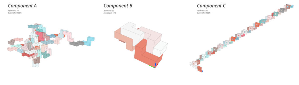
Component Design
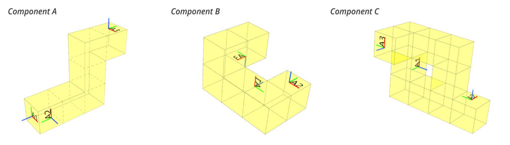
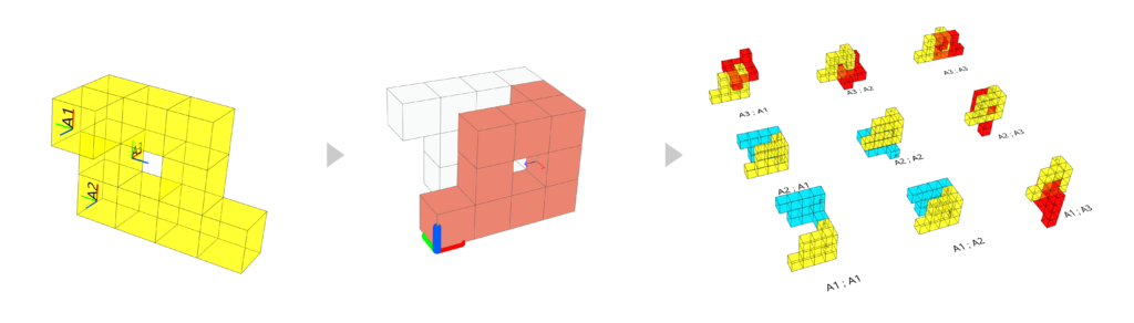
To begin, each of us created multiple voxel-based component designs. Below are three highlighted.
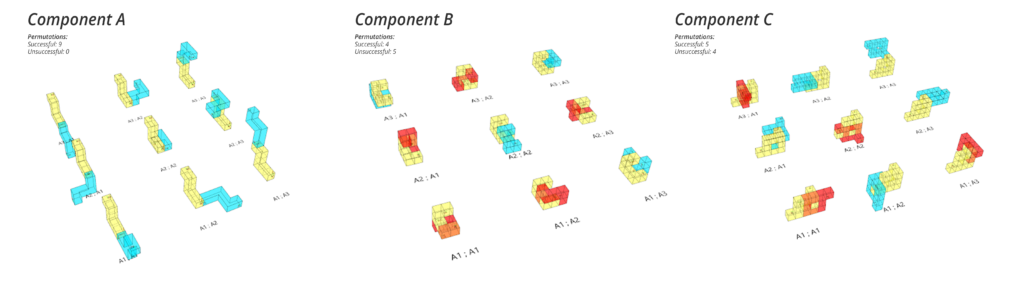
Permutations:
Each component has three connection planes: A1, A2, and A3. These planes serve as connection points for the following combinations. The combinations involve cross-referencing each plane with the others to check for possible intersections. In this case, since we are cross-referencing three handles with each other, it results in 9 combinations. However, due to the placement of the handles, some combinations are unsuccessful as they would intersect with themselves. These unsuccessful combinations are highlighted in red.
Assemblages:
The permutations are related to the development of the Assemblages. An assemblage is created using a loop in Grasshopper through Anemone. The Anemone loop examines the planes of a component and determines how they can be connected to each other. This process is repeated for a specified number of iterations. It also checks if the planes intersect or are obscured, and ensures that they grow above the Z=0 plane. Due to the placement of the handles in the component design and the Anemone script, each assemblage behaves uniquely, as shown below.
Comparisms:
An example of how an assemblage can change is shown below. By simply rotating the A2 plane, the entire assemblage changes completely.
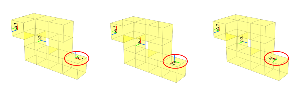
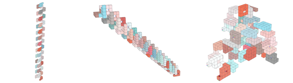
Figure 6: Assemblages created from turned handles
The same effect is also visible when a plane is moved. In the example below, the A2 plane is relocated to different positions to evaluate the various handle placements.
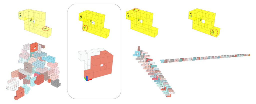
The most unique outcome for us was the second one, with only one successful permutation in the assemblage. We further investigated this and found that it was due to the Handles A1 and A2 blocking other possible intersections and the “Grow Z>=0” command in the script. Below is an example.
Growth Filter
For our custom filter we wanted iteratively add complexity to our script, starting simple and adding complexity along the way.
The basic idea:
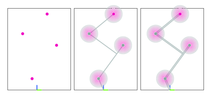
- Generate a a certain amount of randomly placed attractor points (shown in pink below) in 3D Space
- Find the shortest possible path to each of the points
- Grow at the attractor points
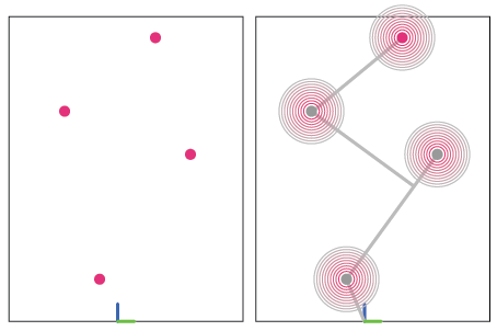
First Attempt:
In the second attempt, we attempted to streamline the script. Visually, the script functioned as pictured below. We generated attractor points, evaluated them by their distance to 0, sorted them, and let the script move the components from point to point. The interesting part came when it reached all the points. The script would then start going through each of the points again, placing one component as close as possible to the attractor point, realizing it is within the threshold of the attractor point and moving on to the next. This had the effect of growing compact around the attractor points.
Second Attempt:
In the second attempt we attempted to streamline the script. Visually the script fuctioned as pictured below. We generated attractor points, evaluated them by their distance to 0, sorted them, and let the script move the components from point to point. The interesting part came when it reached all of the points. The script would then start going through each of the points again, placing one component as close as possible to the attractor point, realizing it is within the threshold of the attractor point and moving on to the next. This had the effect of growing compact around the attractor points.
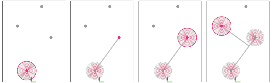
Example:
Below, an example GIF of the code functioning. To test it, we utilized a cuboid shape with three handles. Additionally, we chose only three attractor points, which are depicted by the grey moving circle.
Script:
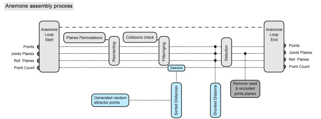
Below is an example of how the Anemone Loop can be used to achieve the animation described above. The gray section represents the loop that was already used in previous assemblies, and the blue additions are the filtering steps. We start by generating a random set of 3D points, sorting them based on their distance from zero, and then passing them through the loop. To accomplish this, we have added an input/output to the loop called “Point Count”. This input/output compares the closest distance of an attractor point with the closest distance of component permutations and dispatches that one. In simpler terms, it checks if the component is moving towards the attractor point and if it is within a certain threshold of it. If both conditions are true, the “Point Count” is incremented, and the next attractor point is selected. This process is then repeated for all the iterations.
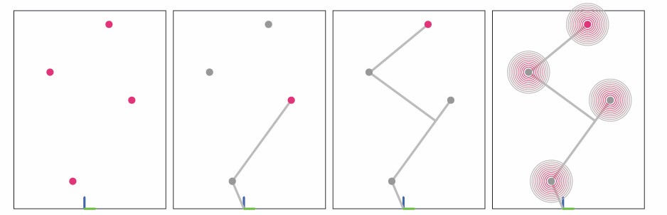
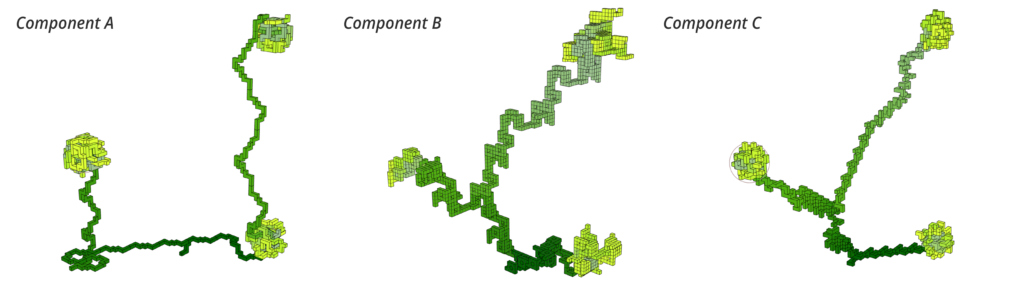
We also applied the script to our components to observe their different behaviors. All components use the same attractor points and the same number of iterations. However, the placement of planes on each component results in a different selection of the shortest path to each attractor point. This also affects the growth around the attractor point, as the compactness is determined by the versatility of the planes in creating a compact volume.
Growth & Compactness Filter
Exploring how to manipulate the shortest path and reward it if it compacts along it.
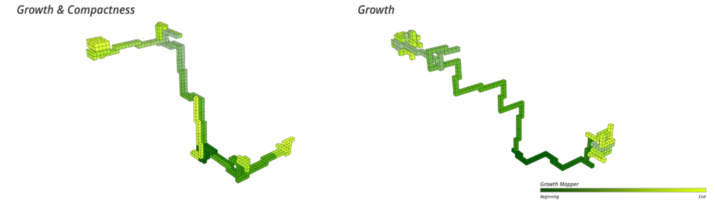
Whilst the previous filter achieved everything we originally set out to achieve, we decided to attempt to control the thickness during the growing phase. As can be seen below. To visualize the growth, the assemblages the assemblage is color-coded, starting with a dark green and transitioning to a light green. The Growth & Compactness filter weights each component based on how close it is to the attractor point, and also how much its placement would add to the volume of the assemblage. The weighting is happening through two values that are customizable.
Script:
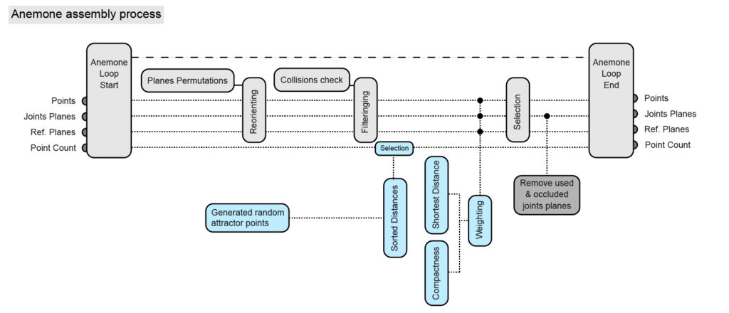
In the Anemone assembly process, the weighing process between the shortest distance and compactness commands is visualized. The loop is otherwise identical to the shortest distance Anemone loop.
Weighting:
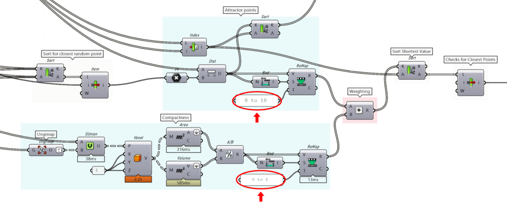
The key aspect of the script is the weighting of the two commands. Below is a screenshot of the Grasshopper logic to highlight the weighting. The two numbers highlighted in red are the values that decide what script has a higher weighting, the attractor points, or compactness. In this case all the values from the attractor point script get remapped between 0 and 10 and the ones from the compactness script 0 to 2. These values then get sorted by the shortest and dispatched according to their original order. In this example, it is evident that the attractor point range is much higher and the numbers generated are also larger numbers. This means that the script will prioritize the attractor point command.
Weighting examples
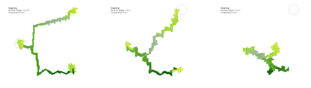
In the figure below, the different weightings are visible. All of them have the same attractor points and 188 iterations. From left to right, the thickness of the growth is changing, and the example on the right does not even reach all the attractor points. The growth and compactness script allows for a high level of control over the assembly, without forcing it to move in a certain way. It simply creates a bias towards one of the options based on the behavior the user wants to enforce. This type of weighting is the basis of machine learning, where choices are reinforced if the network is meeting certain inputs.
The final part of this project was to look at robotic pick and place operations. We assumed that the shape of the block would always come from the same location, and placed it with always picking the top surface of the component. This was just done as an exercise to practice pick and place with the robot, without considering any real world limitations.