
Goal: to predict trip duration of NYC cabs using machine learning models.
Tools: Python + Nympy + Pandas + Datetime + Plotly.express + Matplotlib + Math + Seaborn + Bokeh + Sklearn
Stages of project: data cleaning, data analysis, data preparation, data testing, evaluating prediction accuracy.
Data cleaning
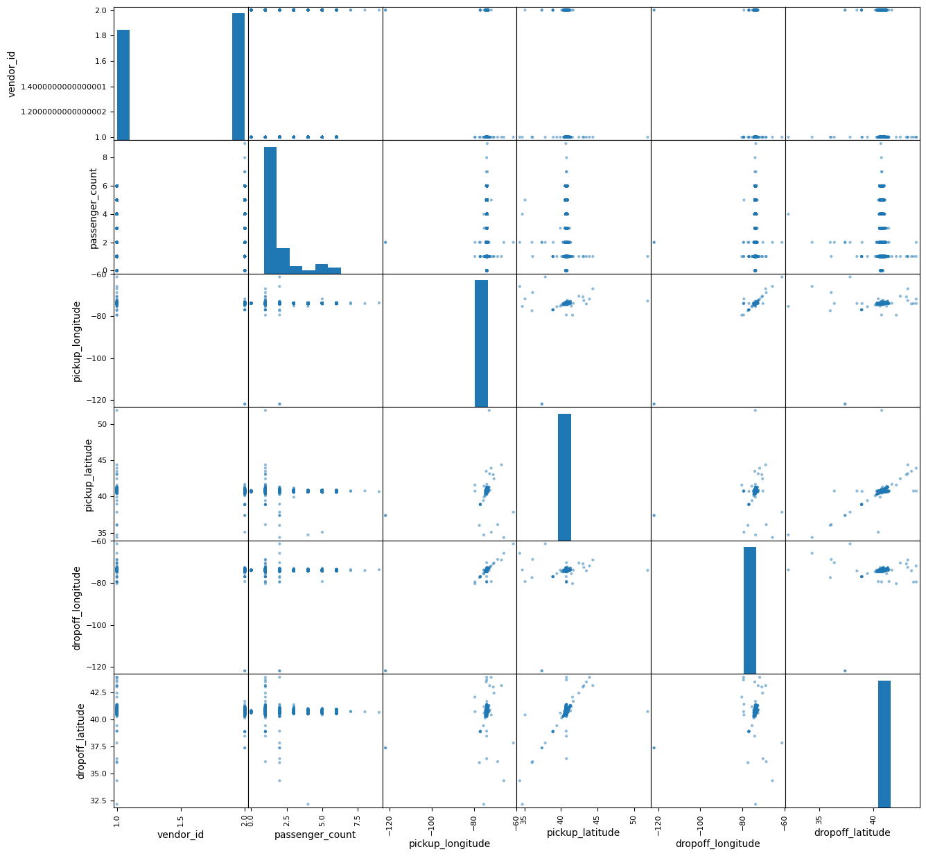
The first dataset visualization with splitting datasets into numeric and categorical and applying the Pearson analysis unveils existing outlayers in time-related and geography-related data.
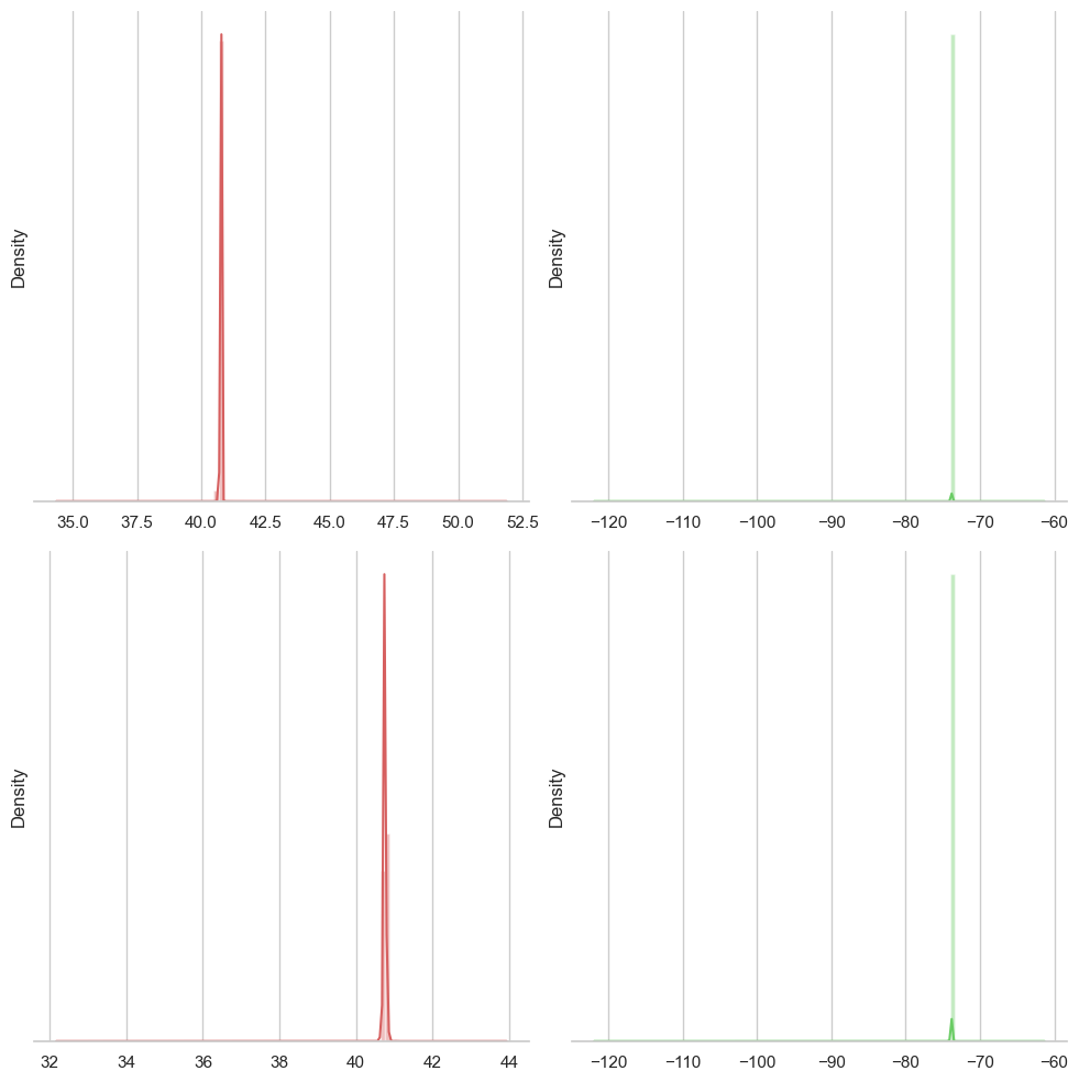
One more visualization analysis of pickup and dropoff geo-coordinates with sns distplot proves existing outlayers in both directions.
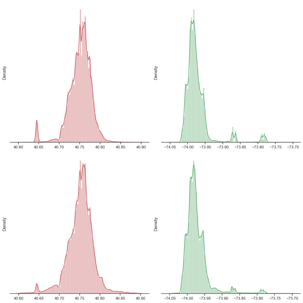
After removal of remote latitude and longitude geo-coordinates framing the dataset to the NYC boundaries, the sns distplot reveals a different picture.
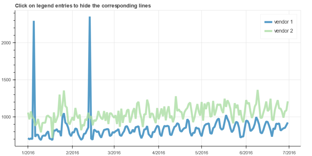
Next, let’s analyze the time-related part of the dataset more precisely. Let’s convert strings to datetime, and make analytical visualization of time data of pickup and dropoff of cab clients by vendors type, and figure out outlayers.
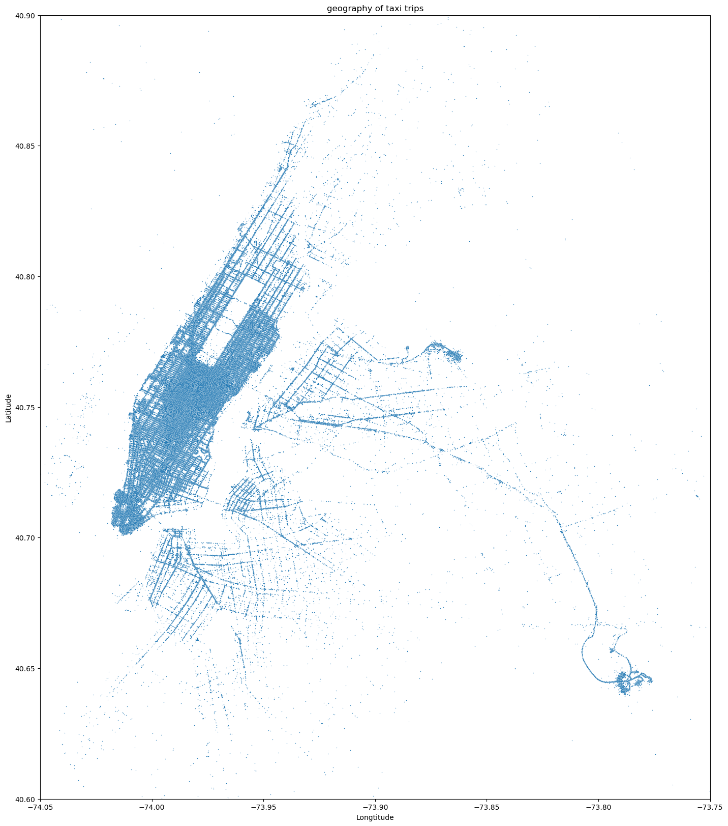
Next step is to clean outlayers of geo-coordinates outside NYC boundary and visualize data on a map with Plotly.
Data analysis
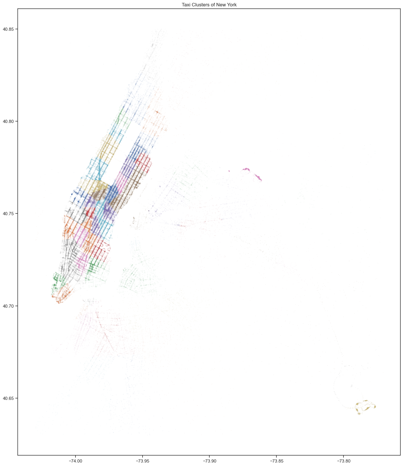
Data analysis starts from a clustering approach of geo-data with KNeighborsClassifier dividing the cleaned dataset into 59 clusters that is equal to the amount of Neighborhood Boards in the New York City.
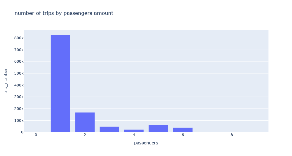
Next step is to analyze the trip frequency with different amount of passengers.
Data preparation
Data preparation includes steps: removal of outlayers of passengers = 0 and > 7, removal of trips longer 3 hours (10800 s), removal of trips beyond the boundary of NYC (-74.03 to -73.75, 40.63 to 40.9).
Evaluation of the share of filtered trips correlates to 99.85%. After that we have to count the difference between pickup and dropoff points of geo-coordinates and add them to the dataframe, and to calculate a distance of 1 degree in km on specific latitude with by Haversine formula (haversine(?) = sin²(?/2)). At the latitude of NYC = 40.5, one degree is equal to 84553 m, and one geo-minute is equal to 1.42126. After that we reduce rows by distance larger one minute, get month, day, hour, day of week from the pickup datetime column, split the dataset to train and test parts.
Data testing
The prediction with Linear regression returns the result of the Median absolute error in seconds = 291.0918991901533.
Next step is to load RandomForest regression and fit the model, load test of the absolute metric error for RandomForest regression, and get prediction for the full dataset.
Evaluating prediction accuracy
R2 score for the prediction evaluates the ratio of 0.7957444370115131.
In order to improve the trained model further we could add more data about weather conditions, data traffic jams, clustering by zipcodes.
