The New York City Taxi Trip Duration competition is a challenge to develop a model that predicts the total ride time of taxi trips in New York City.
Yellow medallion taxicabs, which number 12,779 in New York City, generate a substantial revenue of $1.8 billion per year by providing transportation services to around 240 million passengers. Given their pivotal role in the city’s transportation system and their visibility in Manhattan traffic, data related to taxi trips is of interest to a wide audience. Accurately predicting the duration of taxi trips could offer valuable insights to city planners and the general public of New York, making this problem statement highly significant.
-Data Collection-
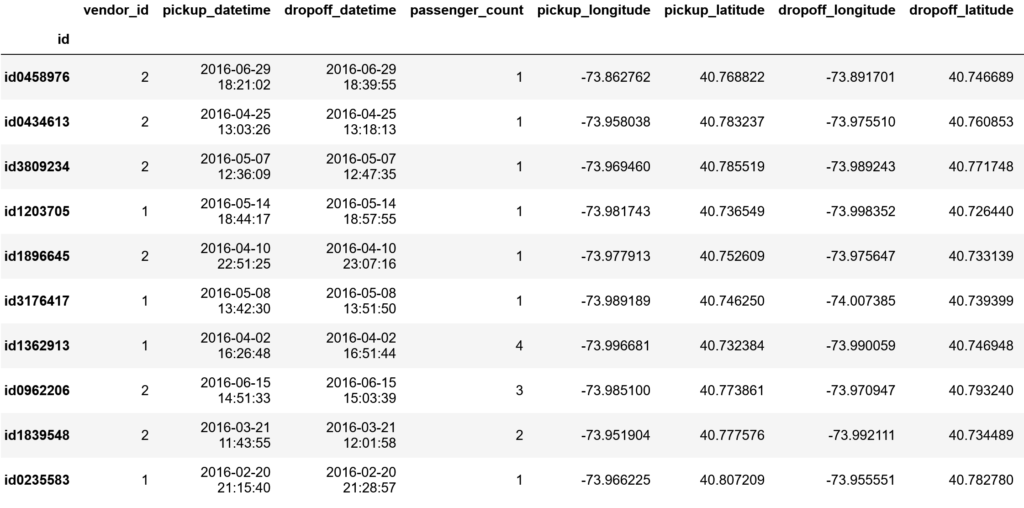
The dataset contains information on over 1 million taxi trips, including 11 features such as the pickup and dropoff locations, pickup and dropoff times, the number of passengers and distance travelled, among others. This first module consisted of having an initial understanding of the data at hand and how each different feature could affect the trip prediction target feature.
-Data Exploration-
Main analysed features
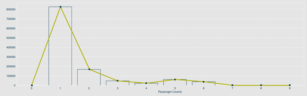
The analysis starts by checking the ‘passenger_count‘ feature, visualising it with value counts plot and list. The study reflects many trips are taken by 1 to 6 people.
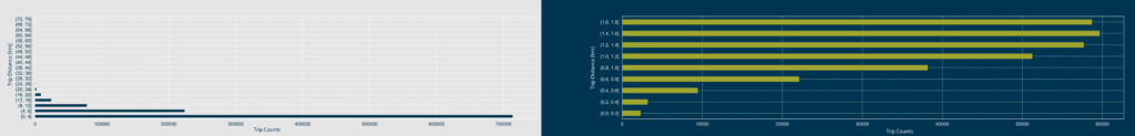
Next, the target feature ‘trip_duration‘ is investigated. Most of the trips have a duration between 0 and 60-70 minutes. To be more precise in the short trips and detect outliers, the trip_duration is grouped into intervals of 1 minute to plot a horizontal bar chart. By doing so, it is revealed that around 20k trips are below 2 minutes, which are too short to be taken into consideration.

The ‘distance‘ between pickups and dropoffs is another important feature to consider in predicting the trip duration. To be more precise in the calculation of the distance, the “Manhattan distance” is calculated (distance between two points measured along axes at right angles). The calculated “Manhattan distance” is stored in a new column named “trip_distance_manhattan_km.” By analysing the results, it is revealed that most of the trips cover a distance between 0 and 32 kilometres. Again, to detect outliers in short trips, the trip_distance_manhattan_km is grouped into intervals of 0.1 km to plot a horizontal bar chart.
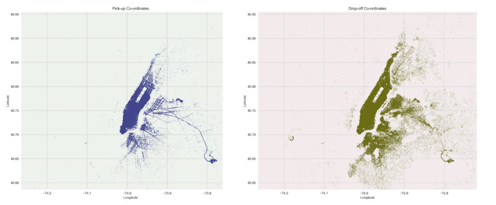
Moreover, to prove the concentration of trips in a radius within the range mentioned above, ‘pickups, and dropoffs‘ are plotted on the map of Manhattan. It is observed that pickups are more concentrated than dropoffs, but they still match the 5 km distance. Moreover, the maximum distances are around 30 km, which are consistent with the results of the trip_distance_manhattan_km horizontal bar chart.
Considering the trip_distance is concentrated in a range of circa 30km, I proceed to analyse the given coordinates for pickup-dropoff locations in NY as there could be outliers in these features too.

-Feature Engineering-
–Removing outliers–
According to the exploration and understanding of the data, outliers will be dropped in the following features:
>Passenger Count: Trips with passenger counts outside the range (1, 6) are dropped as they might cause distortion in the process. I follow checking the trip duration feature, which is the target feature.
>Trip Duration: Trips shorter than 3 minutes and longer than 60 minutes are removed.
>Trip Distance: Trips covering less than 500 meters are removed from the DataFrame to ensure consistency with the cleaning in the trip_duration feature.
>Pickup-Dropoff Coordinates: The charts above show a concentration of latitude and longitudes that confirm the existence of outliers to either end. Following the same principles timeframe (3-60 min) and distance (0.5-50km), I clean cleaning outliers of the coordinates feature.
–Dropping useless features–
The following columns are removed due to its lack of importance for the prediction:
>id : Set as index
>vendor_id
>store_and_fwd_flag
–Feature Extraction/Transformation–
Firstly, I convert the ‘pickup_datetime’ feature to a datetime type to extract useful features, such as the hour, month, day of the week, and weekday-weekend indicator. Methods such as “strftime”, “normalize” and “dayofweek” are used for extraction and creation of new features.
Similarly, features are extracted from the ‘dropoff_datetime’ feature, such as the month, hour, and day of the week, creating new columns to the “df_train” dataframe.
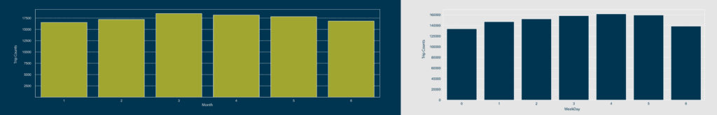
To understand the distribution of the trips per weekday and per month, two count plots are created using the “sns.countplot” method, along with the “plt” module. These plots show that the demand for taxis is increasing from Monday to Friday and that the distribution of trips is relatively even across the different months (above chart). Finally, based on the analysis of the above plots, the “is_WeekDay-Weekend” feature is not considered as individual days might give more specific insights for future prediction.
In regards to the process of scaling features, I choose a Normalisation to make the dataframe evenly distributed and lighter, but the results of the prediction are not altered significantly. Therefore this transformation will not be considered.
After all, the features that conform that final dataset are: passenger_count, pickup_longitude, pickup_latitude, dropoff_longitude, dropoff_latitude, trip_duration, trip_distance_manhattan_km, pickup_hour, pickup_month, pickup_day_of_week, dropoff_month, dropoff_hour, and dropoff_day_of_week.
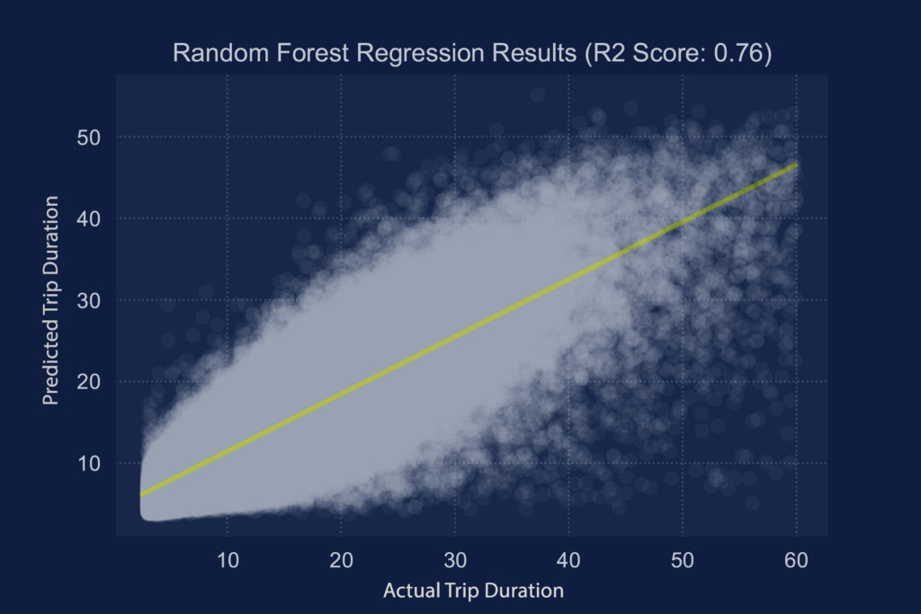
-Model Selection & Training-
This step consists in using the selected predictive model to learn from the data and adjust its parameters to optimize its performance. I proceed by splitting the dataset into training and validation sets (random split of 20%test-80%train), using the training set to train the model and the validation set to evaluate its performance. I experimented with various machine learning algorithms, including linear regression, decision trees, and random forests, being the latter the most consistent one. Lastly, to evaluate the quality of fit of the regression model, I use the R-Squared measure, obtaining a final score of the prediction of R2=0.755.