
“Can we understand urban environments and street characteristics from Google Street View panorama images using Machine Learning and Stable Diffusion techniques?”
Project Overview
This computational design project aims to develop a pipeline utilizing Grasshopper and Python to visualize clusters of panoramic streetscape images. The project leverages t-Distributed Stochastic Neighbor Embedding (t-SNE) for dimensionality reduction, facilitating the identification and analysis of patterns within the streetscape imagery. By clustering these images, we can gain insights into the visual characteristics and urban patterns of different neighborhoods.
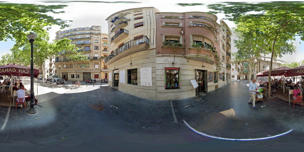
STREET ANALYSIS is a tool that helps explore and understand streetscape better. By using Google Street View images and machine learning, it allows users to select areas of interest and access detailed street information. From defining study areas to analyzing street characteristic. STREET ANALYSIS offers an experimental way to explore the street pattern in urban environments.
METHODOLOGY
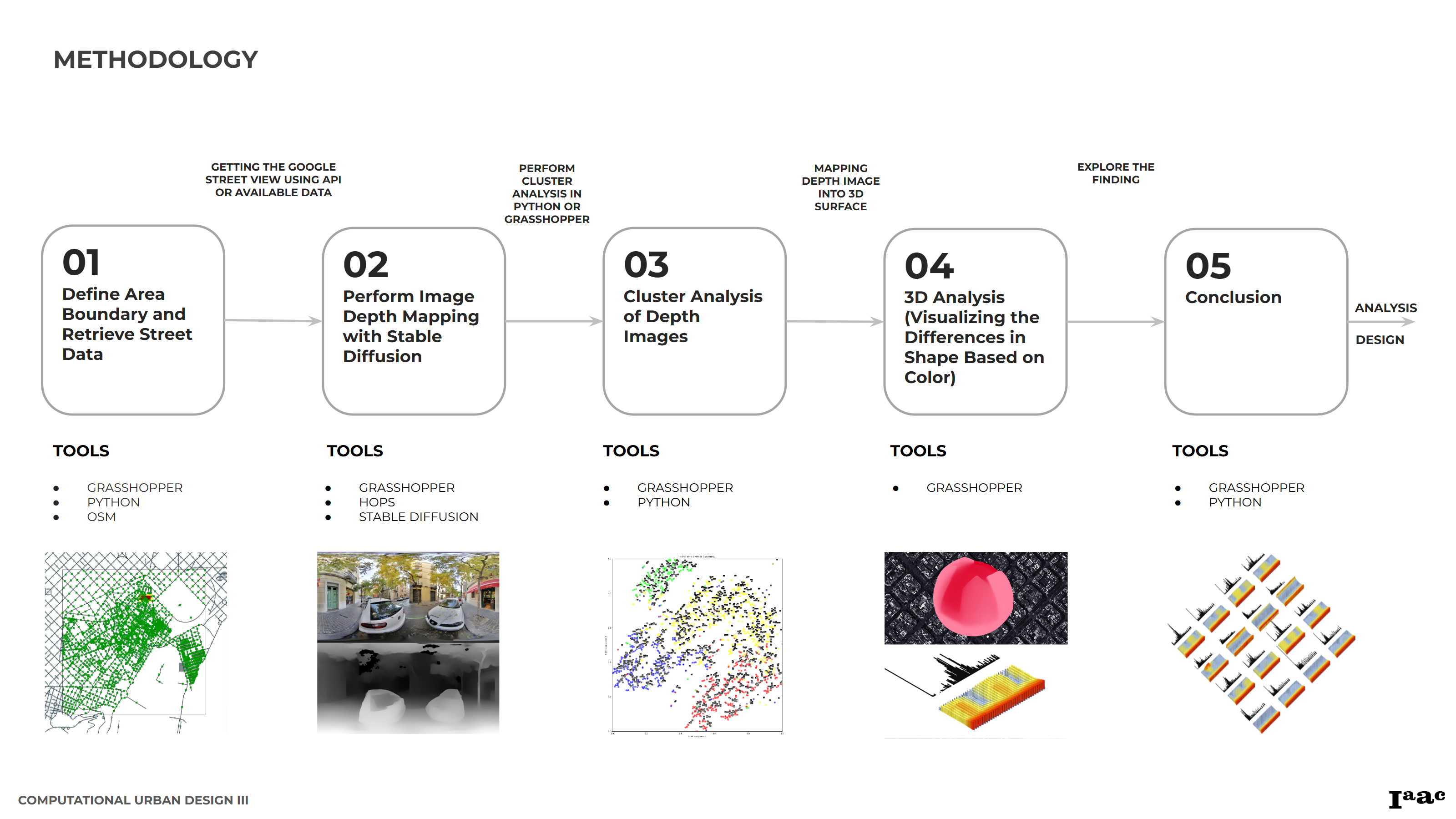
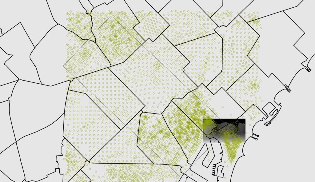
1. Defined Area and Data Gathering
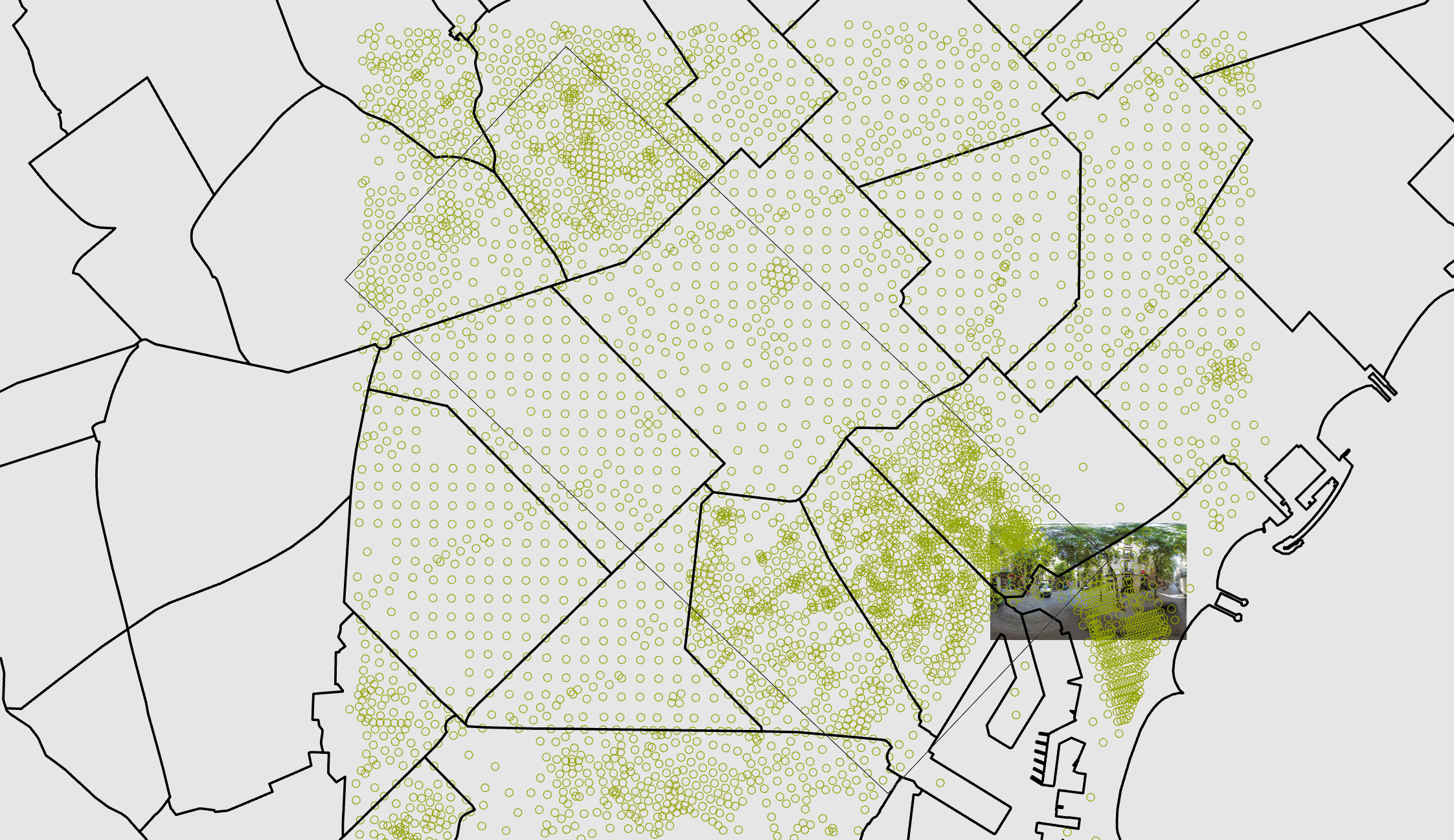
The first step in our process is to define the area for analysis and gather the necessary data. Users can select any area for street analysis using Python and Grasshopper. Here’s how it works:
- Area Selection:
- Python Script: We create a Python script that allows users to select a boundary area based on coordinates. This script identifies the center points of streets and coordinates from OpenStreetMap (OSM).
- API Request: Using these coordinates, the script requests Google Street View data via an API. Note that accessing Google Street View data may require payment, so in this example, we use a dataset provided in class.
- Required Inputs:
- Google Street Panorama Images: Images with filenames for reference.
- Shapefile of Streets: A shapefile representing the streets in the study area.
- CSV File: A CSV file containing x and y coordinates and corresponding image codes.
- Integration with Grasshopper:
- In Grasshopper, these inputs are connected and mapped to visualize the street images on a map.
- Users can crop specific boundary areas for focused study, and the image paths are then sent to the next process for depth analysis.
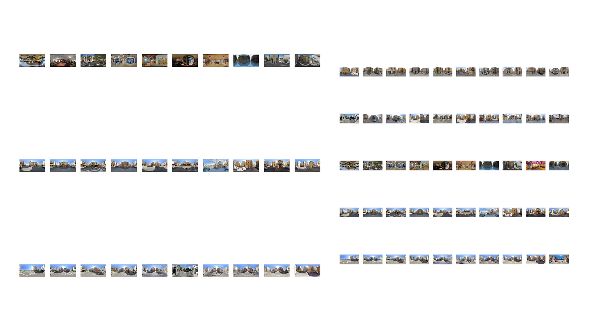
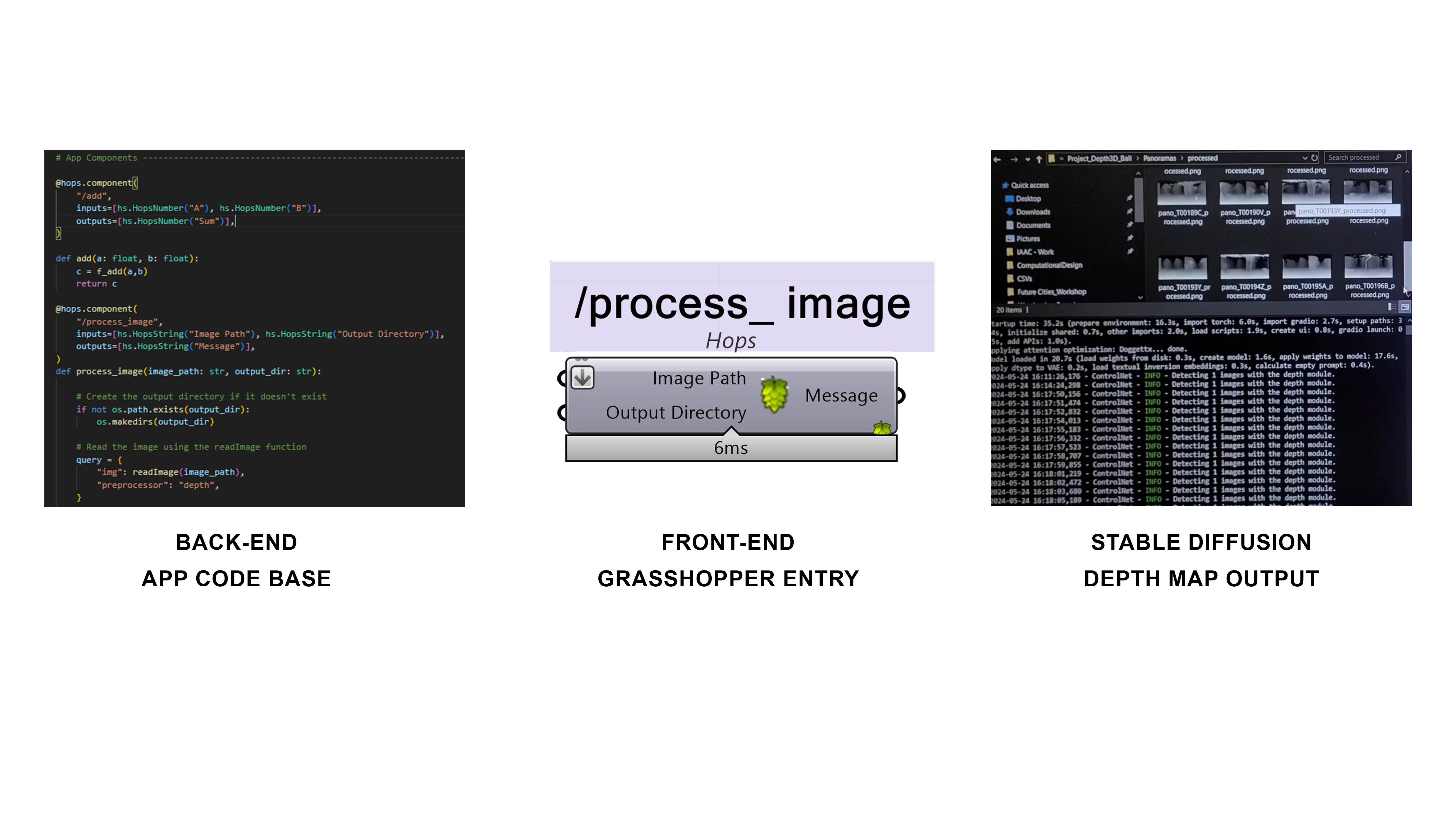
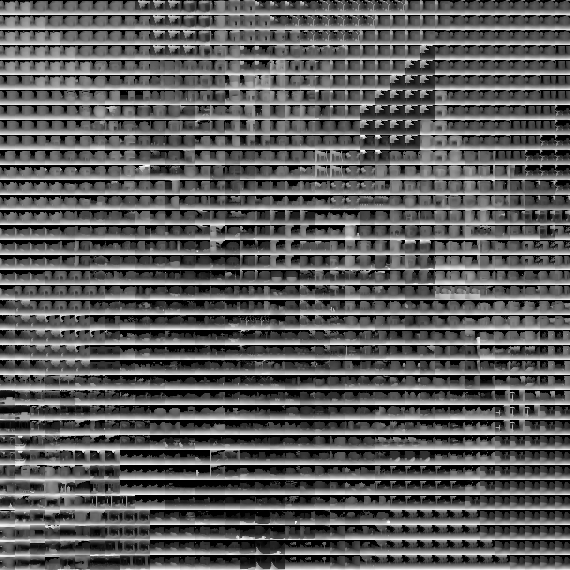
2. Depth image processing
An exposed API connection using stable diffusion through the frameworks of A1111, we can effectively transform panoramic street images into depth images. This process involves the following steps:
- Conversion Process: The ControlNet (Midas) tool analyzes the color image and converts it into a depth image. In the depth image, lighter shades (closer to white) indicate objects nearer to the camera, while darker shades (closer to black) represent objects further away. This objectively indicates elements in the panorama that are closer and further away from the center of the street.
- Applications: These depth images help in understanding the spatial arrangement and distances within the 2D images, providing a pseudo-3D perspective that can be crucial for various analyses.
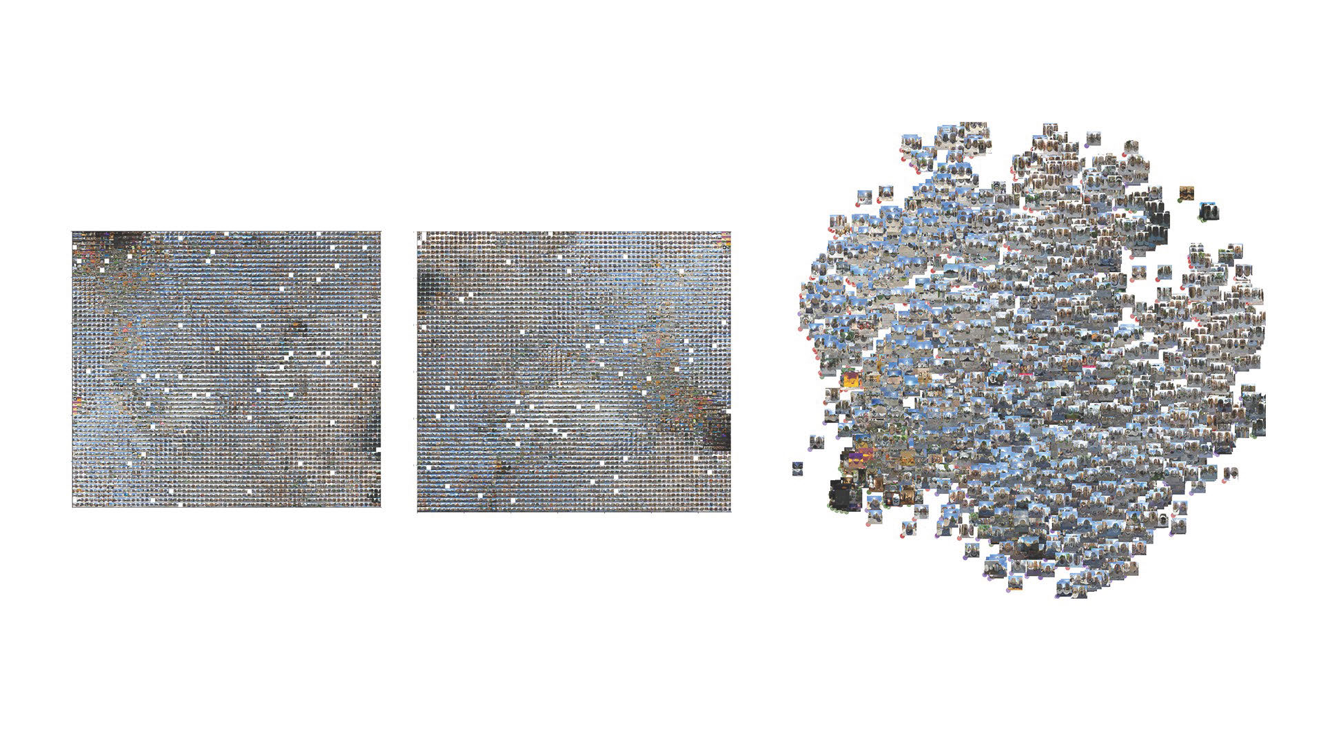
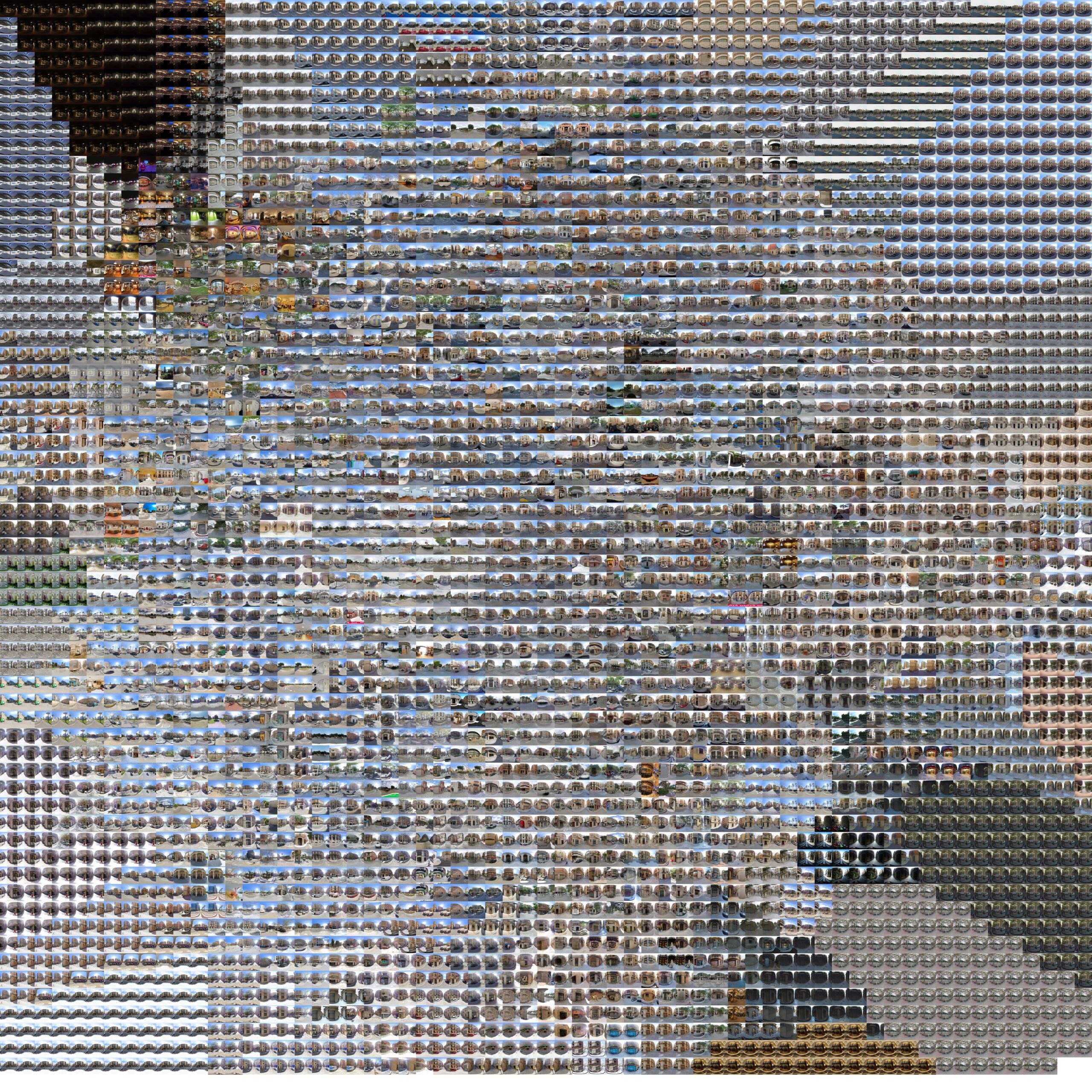
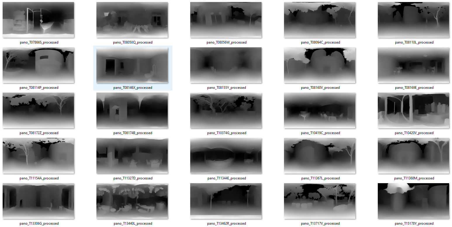
3. Images clustering
The depth images were then clustered using t-SNE for dimensionality reduction and K-Means clustering, with the optimal number of clusters determined by silhouette scoring. The script allowed for either user-defined clustering or automated determination of cluster count based on dataset analysis. Finally, the clustered images were saved into directories corresponding to their cluster labels, facilitating the analysis of street characteristics and distribution across the city.
The data collection involved gathering and pre-processing the substantial dataset of panoramic urban streetscape images from each neighborhood (barrio) of Barcelona.
Once we have our depth images, the next step is to analyze and cluster these images to identify patterns and group similar images together. This is where Python and machine learning techniques come into play:
- Analysis Using Python: We use Python scripts to read the depth images from a directory and perform clustering analysis.
- Clustering with t-SNE: By employing machine learning algorithms like t-SNE (t-Distributed Stochastic Neighbor Embedding), we can visualize and cluster the depth images accurately. This helps in identifying distinct groups based on the depth information.
- User-defined Clustering: Users can set the number of expected clusters, and the Python script will automatically calculate and separate the images into the specified groups. The clustered images are then saved into respective directories.
4. 3D analysis and visualizing
By interpreting the bar graph, users can understand the distribution of distances in the depth image. For instance, if most bars are tall in the lower range (0-30 meters), it indicates that many objects in the scene are close to the camera. Conversely, if the taller bars are in the higher range (70-100 meters), most objects are far from the camera.
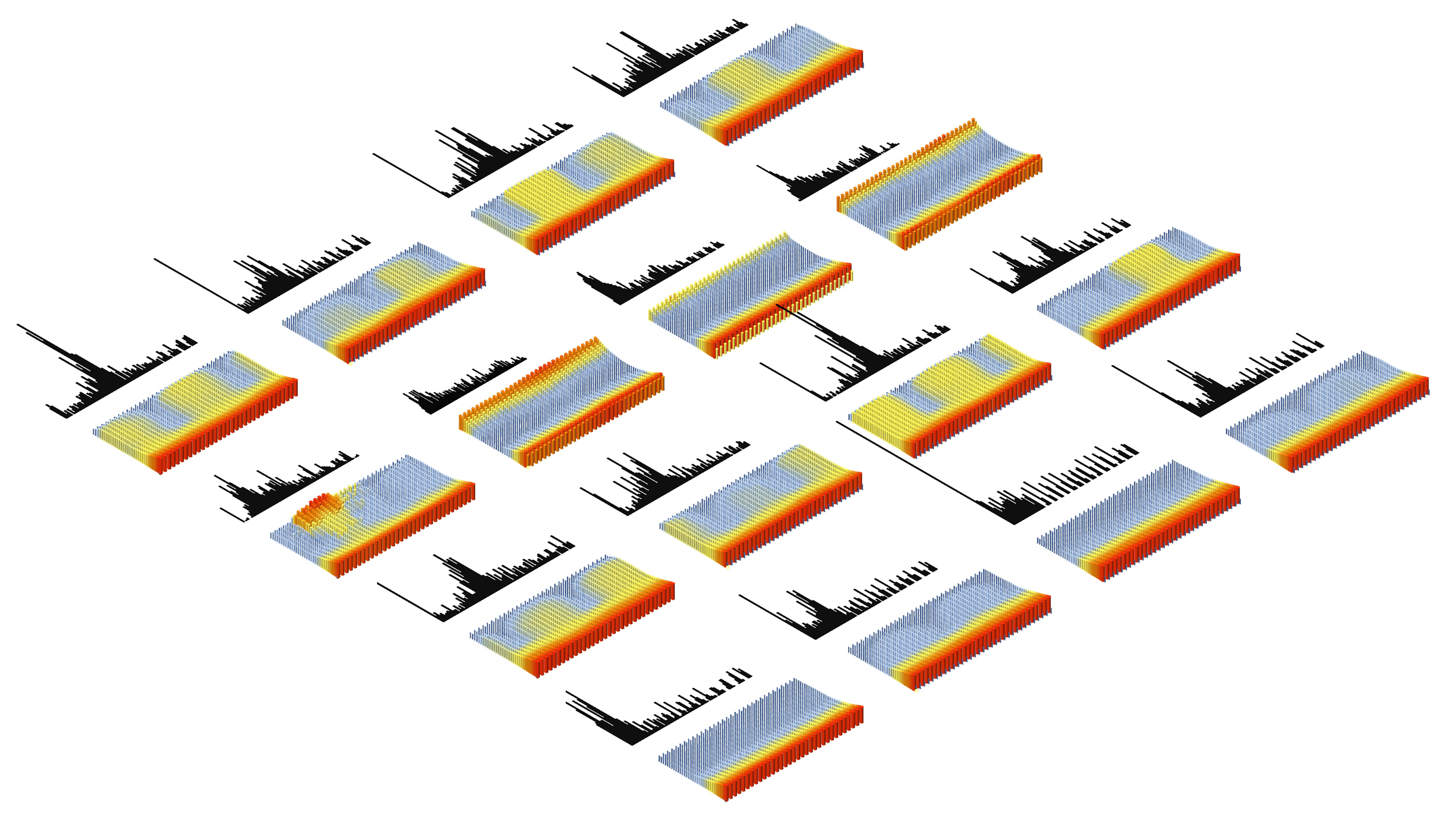
Interpreting the x and y axes of a depth image bar graph in terms of street quality or other practical metrics can provide valuable insights into the urban environment. Here’s how you might relate these axes to aspects of street quality or other contextual information:
X-Axis (Horizontal):
- Depth Value Bins: The x-axis represents bins of depth values, which indicate the distance from the camera to objects in the scene. In terms of street quality, these depth values can be related to various elements such as:
- Pedestrian Pathways: Depth values indicating the proximity of sidewalks or pedestrian zones.
- Street Furniture: Distance to objects like benches, trash bins, and other street furniture.
- Building Fronts: The proximity of building facades to the street.
- Vegetation: The distance to trees, bushes, and other greenery, which can contribute to the aesthetic and environmental quality of the street.
Y-Axis (Vertical):
- Frequency/Count: The y-axis shows the number of pixels that fall within each depth value bin. This can be interpreted to reflect the density or prevalence of certain features within the depth ranges:
- Street Clutter: High counts in certain depth bins may indicate clutter or congestion, such as parked cars or dense street furniture.
- Open Spaces: Lower counts in specific depth bins can indicate open spaces, which might be desirable for pedestrian areas.
- Uniformity: The distribution pattern can reflect how uniform the street layout is; a very varied distribution might indicate a mix of open and obstructed areas, while a more uniform distribution could indicate consistent building setbacks or street widths.
5. Conclusion
Example Interpretation in Terms of Street Quality:
- Even Distribution of Depth Values:
- Implication: An even distribution of depth values across bins might suggest a well-planned street with consistent building setbacks and well-placed street furniture, contributing to a balanced urban environment.
- Street Quality: Likely high, indicating good urban planning and accessibility.
- High Frequency in Short Depth Ranges:
- Implication: A high frequency of pixels in short depth ranges (closer objects) could indicate narrow streets, closely packed buildings, or excessive street furniture.
- Street Quality: Might indicate lower quality in terms of open space and pedestrian comfort, but could also reflect a vibrant, densely populated urban area.
- High Frequency in Long Depth Ranges:
- Implication: A high frequency of pixels in longer depth ranges (farther objects) suggests more open space or wider streets.
- Street Quality: Could be positive, indicating spaciousness and better airflow, but if too sparse, might lack street activity and vibrancy.
This project demonstrates the integration of geospatial data collection, advanced image processing, and machine learning techniques to analyze urban street environments. The resulting visualizations and data analyses provide valuable insights into the city’s street characteristics and distribution, supporting urban planning and development efforts.
