ABSTRACT
The integration of generative AI into architecture is transforming early-stage design processes, particularly by enabling rapid and automated floorplan generation. These tools increase efficiency by exploring large design spaces and producing multiple layout options in a short time. However, current workflows struggle to integrate critical performative analyses such as daylight availability, thermal comfort, and energy demand into the earliest phases of design. The absence of integrated performance feedback at the stage where design decisions have the greatest impact risks overlooking important optimization opportunities.
Most existing datasets for automated architectural design are limited in scope. Many are synthetic rather than based on real-world buildings, which introduces a garbage in garbage out risk when models are trained only on generated floorplans. Furthermore, no publicly available datasets combine architectural layouts with geocoded information, climate data, and energy simulations, even though building performance is deeply tied to location and environmental context.
This project develops a real-world architectural dataset enriched with geospatial information (GeoJSON), environmental data, and energy simulation outputs. The dataset provides a foundation for advancing performance-informed generative design, enabling machine learning models and design tools to account for climatic and geographic conditions alongside spatial and geometric qualities of buildings.
#01 INTRODUCTION
CONTEXT
The integration of AI is reshaping the early design stage in architecture—particularly through automated floorplan generation that can explore large design spaces and produce numerous alternatives rapidly. This capability is well documented in recent reviews and case studies, but most tools still privilege speed and spatial feasibility over performance, unless performance analysis is explicitly integrated into the workflow (Weber, Mueller, & Reinhart, 2022; Meselhy et al., 2025).
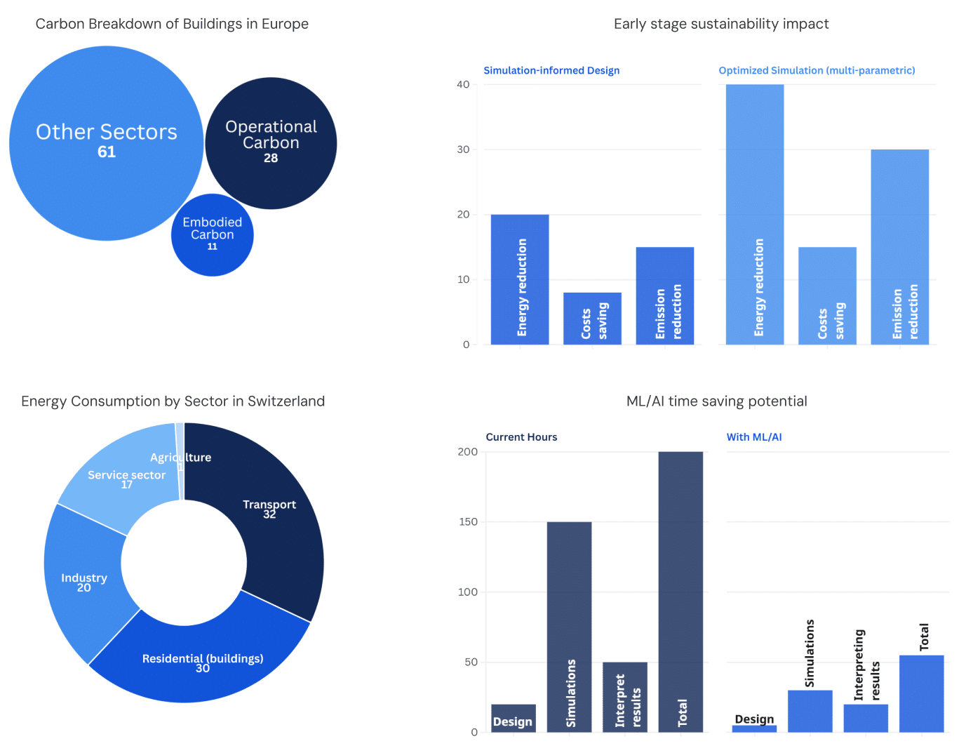
The stakes are high: buildings account for roughly a third of EU greenhouse-gas emissions (European Commission, 2020; World Green Building Council, 2019). At the same time, residential buildings alone consume about 28–30% of Switzerland’s total final energy, so even modest efficiency gains at scale matter (IEA, 2025).
Critically, decisions made in the earliest design stages have the greatest leverage over lifecycle performance and costs, which is why bringing performance data forward is essential (Bragança, Vieira, & Andrade, 2014; Ouldja et al., 2024).
ML approaches can make this practical: surrogate models now predict key performance metrics in milliseconds, enabling orders-of-magnitude more iterations and faster feedback loops than conventional simulations (Wang, Harrison, Teigland, & Hollberg, 2024; Singh, Deb, & Geyer, 2022).
PROBLEM STATEMENT & RESEARCH QUESTION
Despite rapid advances in AI-assisted floorplan generation, most tools still optimize for speed and quantity rather than for how a layout actually performs (e.g., daylight & energy consumption). As a result, early design alternatives are often selected without quantified performance feedback—precisely when design decisions have the greatest leverage over lifecycle outcomes (Bragança et al., 2014; Weber et al., 2022).
In practice, high-fidelity simulations struggle to keep pace with the hundreds of options AI can generate; reviews call out early-stage simulation as computationally demanding, motivating the use of surrogate/ML models to deliver rapid, credible feedback (Østergård et al., 2016; Westermann & Evins, 2019; Wang et al., 2024). Site and urban-context effects (climate, shading, surrounding massing) are also not systematically integrated into early workflows even though they influence results (Reinhart & Cerezo Davila, 2016; Hong et al., 2020).
This thesis addresses that gap by proposing a scalable workflow to enrich floorplan datasets with context-aware performance attributes so designers and future ML models can compare and select performance-aware layouts from the very first iterations. This leads to the central question:
How can we create a workflow to enrich existing floorplan databases with performative data?
HYPOTHESIS
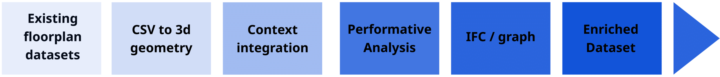
By connecting existing workflows from floorplan to performative analysis, we can create a semi automated pipeline that enhances floorplan datasets with performative data. Our proposed workflow includes acquiring a floorplan dataset, raster-to-vector conversion, generating a 3D model, integrating site context, and running performance analyses.
STATE OF THE ART
The application of generative AI and machine learning in architecture has expanded significantly in recent years, particularly in the domain of automated floorplan generation. Models based on generative adversarial networks, diffusion methods, and graph representations have been developed to produce architectural layouts that satisfy functional and spatial constraints (Nauata et al., 2021; Shabani et al., 2023; Hu et al., 2020). For example, Graph2Plan, trained on the RPLAN dataset of approximately 80,000 annotated floorplans, demonstrates how neural networks can translate abstract spatial graphs into coherent architectural layouts. These approaches illustrate the potential of AI to accelerate early-stage design exploration, but they often remain disconnected from performance considerations such as daylight, thermal comfort, and energy demand (Weber et al., 2022).
Several tools aim to bridge this gap by integrating intelligent design support into the early phases of architecture. Finch 3D is an example of a commercial platform that applies AI-driven optimization and provides feedback on design decisions, offering real-time support for architects (Finch, n.d.). While such tools highlight the potential of combining generative methods with performance analysis, their methodologies and data foundations are often proprietary and lack transparency, limiting their academic reproducibility (Weber et al., 2022).
Datasets are a central driver of innovation in generative design research. MLSTRUCT-FP offers 954 annotated floorplans with polygonal representations of architectural elements, enabling machine learning tasks such as layout parsing and segmentation. CubiCasa5K provides approximately 5,000 annotated floorplan images with detailed room and object categories, supporting tasks in floorplan recognition and generation. More recently, the WAFFLE dataset introduced nearly 20,000 floorplans collected from diverse global sources, reflecting stylistic and cultural variety (Ganon et al., 2025).
At a larger scale, ReCo contains more than 37,000 community layout plans and nearly 600,000 residential buildings with height information, enabling research at the neighborhood and settlement level (Chen et al., 2023). Additionally, specialized datasets such as the Modified Swiss Dwellings dataset offer thousands of apartment layouts that capture the complexity of multi-unit housing (van Engelenburg et al., 2024; Standfest et al., 2022).
Beyond architectural datasets, building performance databases and simulation platforms play an important role in energy and environmental research. For instance, the U.S. Building Performance Database (BPD) provides energy use intensity and performance data for hundreds of thousands of buildings. Meanwhile, tools such as EnergyPlus, OpenStudio, and IDA ICE are widely adopted for simulating thermal performance, daylight availability, and energy demand (DOE, 2024; NREL, 2025; EQUA, n.d.). However, these resources remain separate from datasets used in generative design research, and they typically operate at different stages of the design process.
What remains largely missing is an integrated dataset that combines architectural layouts with geospatial information, climate context, and building performance simulation results. Existing floorplan datasets are either synthetic or limited to geometric annotations, with little or no connection to environmental data. Conversely, energy simulation databases are rich in performance metrics but lack spatial and geometric descriptions of building layouts. This disconnect highlights a gap in current research: the absence of comprehensive datasets that enable performance-informed generative design in architecture (Weber et al., 2022; Chen et al., 2023).
#02 RESEARCH
This chapter summarizes the research that set the pipeline’s requirements and tool choices. We first surveyed open datasets and selection criteria—licensing, geometric granularity (room/door/window), stable IDs, and extensibility—which led us to Swiss Dwellings as the most reliable backbone. We then reviewed ways to convert plans into computable geometry (CV-based raster-to-vector, polygonal parsers, parametric reconstruction) and, after testing options, specified a Grasshopper reconstruction that guarantees clean storey frames and joinable identifiers.
For context integration, we compared open sources and adopted a Cityweft-based workflow to import urban meshes and bind EPW files. Finally, we evaluated simulation platforms and converged on Ladybug Tools for daylight and solar analyses run directly on the GH model (with consistent grids/tolerances), keeping energy modeling as future work. Together, these investigations fixed the project’s fundamentals: the data model (IDs, schemas), the sources of truth (GH for sims; IFC as enriched snapshot), and the export targets (CSV/XLSX, IFC, and graphs).
DATASETS
We began our research by reviewing open datasets that could support architectural machine learning. Our focus was on floorplan collections that were publicly available, well-structured, and suitable for workflows in Rhino and Grasshopper. One of the first datasets we examined was CubiCasa5K, which contains 5,000 annotated floorplans with room and object categories. Its detailed semantic labeling makes it useful for computer vision tasks such as segmentation and classification. However, the data is primarily provided as images, limiting its direct use in 3D workflows.
We also explored Floorplan Masks available on Hugging Face, which provide pixel-level masks for layouts. While valuable for training segmentation models, these datasets remain in raster form and require vectorization before they can be applied.
The Swiss Dwellings dataset and its extension, the Modified Swiss Dwellings dataset, offered more complex layouts with thousands of apartments and multi-unit buildings, providing better diversity and a closer connection to real architectural conditions. Yet, they still lack geospatial and environmental data.
Another dataset we evaluated was the Pseudo Floorplan 12k, which contains around twelve thousand synthetic layouts. Although it demonstrates large-scale generation, its synthetic nature risks introducing biases, as models trained on it tend to reproduce the assumptions built into the dataset.
In addition to open datasets, we examined architectural project databases from websites such as ArchiAlly, Archello, Nextroom, and Building Types Online. These platforms maintain structured project data, including floorplans, metadata, and building attributes, but are not open-source and collaboration was not possible. Since our project aimed to produce an open dataset, we excluded these resources.
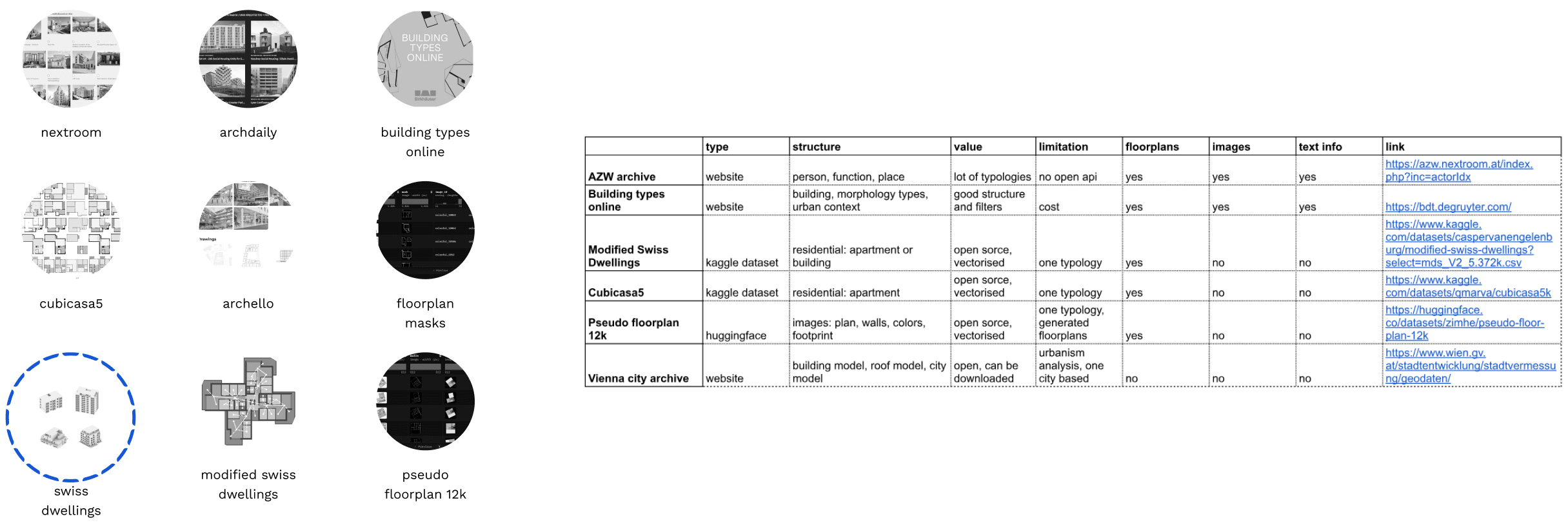
From this exploration, we concluded that most available datasets are designed for computer vision and distributed as images rather than vectorized models, limiting their usability for simulation and parametric workflows. This motivated us to try to define a workflow capable of vectorizing, standardizing, and extending data into formats suitable for 3D modeling and environmental simulation.
While reviewing the datasets, we realized that the Swiss Dwellings dataset could serve as a solid foundation for our project. Its detailed layouts and multi-unit building structures provide real-world complexity, and it could be combined with our own contextual data, such as geolocation and environmental information.
VECTORIZATION
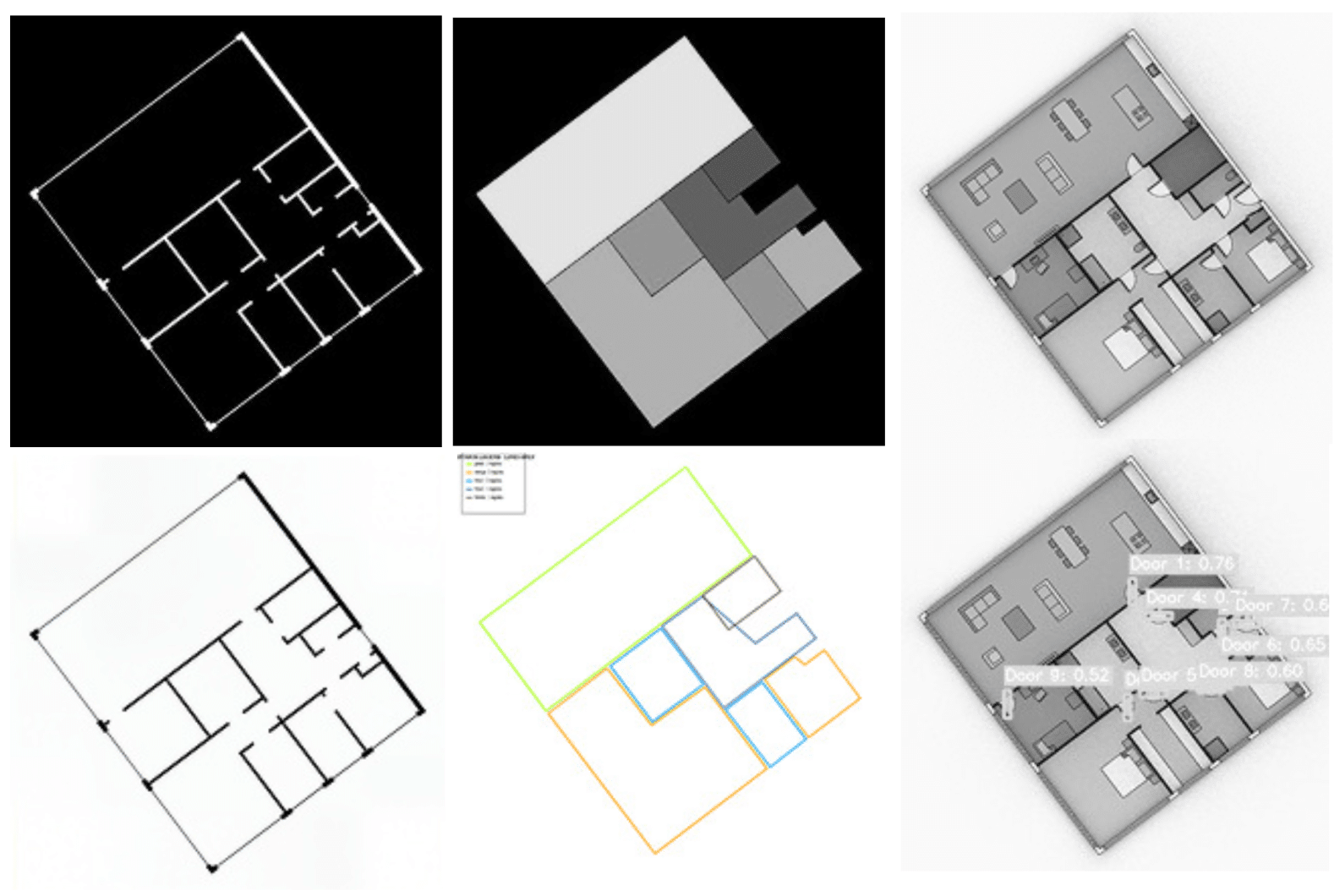
For the vectorization process, we used the Pseudo Floorplan 12k dataset as an example (link). The process began by extracting black-and-white masks of the floorplans. To enhance image quality, we applied the InvSR model (link) and then inverted image channels using PineTools. The enhanced images were vectorized using Vectorizer-AI (link), primarily for extracting wall geometries.
For room types, we generated PNG images and extracted outlines of each color group, exported them as SVG, and imported them into Grasshopper. Door locations were obtained using a Roboflow door detection model, which produced rectangles corresponding to door positions. All these preprocessing steps, including image enhancement, vectorization, and model-based detection, were performed in Visual Studio.
2D TO 3D
Once the SVG files were prepared, they were imported into Rhino and referenced in Grasshopper. We developed a workflow that combined the three SVG types—walls, room types, and doors—while performing data cleaning, line intersection, and alignment operations. This combination formed the basis for generating 3D IFC-ready models.
This workflow, however, was limited to the Pseudo Floorplan 12k dataset. Its scope was restricted to apartment-level floorplans rather than entire buildings, which made controlling the process more challenging. Despite these limitations, the workflow demonstrated a clear pipeline from raster images to 3D parametric models suitable for simulation and further analysis.
Images on the left represent initial pngs and developed model in the end.
CONTEXTUAL DATA
To enhance our architectural models with real-world context, we explored various sources for integrating environmental data. A key resource was Cityweft, a platform designed to provide high-quality 3D city models tailored for architecture, engineering, and construction (AEC) workflows. Cityweft aggregates data from over 150 global sources, including government datasets, LiDAR surveys, and machine learning-derived models, offering editable 3D geometry and terrain data. This integration facilitated the inclusion of accurate building geometries..
In addition to Cityweft, we considered OpenStreetMap (OSM), a collaborative project that provides freely accessible geospatial data. While OSM offers extensive coverage, its data is often less structured and may require additional processing to align with our modeling standards.
Our primary objective was to incorporate contextual data that would enable comprehensive environmental analysis. By integrating these datasets into our workflow, we aimed to create models that not only represent architectural elements but also their surrounding environment. This approach ensures that our simulations account for real-world variables, enhancing the accuracy and relevance of our analyses.
CLIMATE
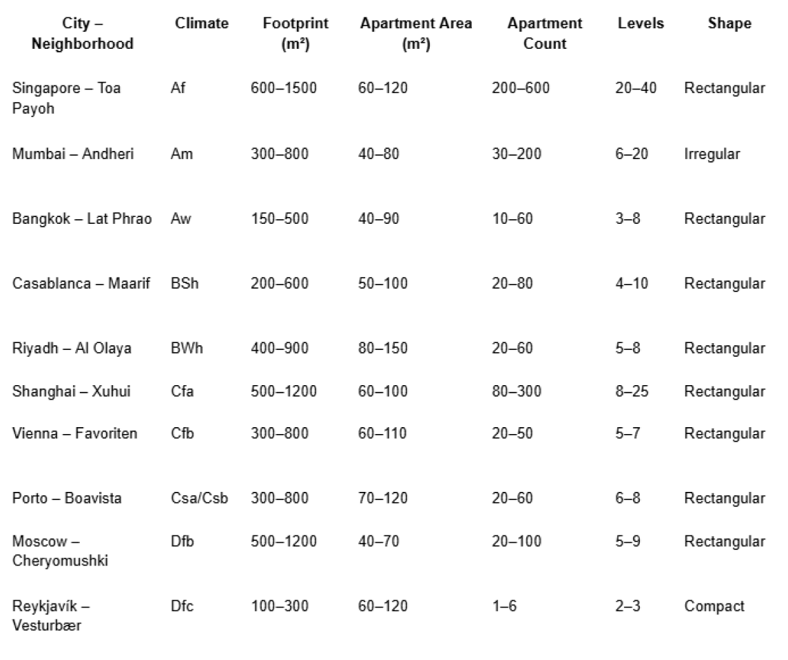
To evaluate the environmental performance of our models, we selected ten cities in the Northern Hemisphere, each representing a distinct climate type according to the Köppen-Geiger classification system. The chosen locations and their neighborhoods are: Singapore – Toa Payoh (Af, tropical rainforest), Mumbai – Andheri (Am, tropical monsoon), Bangkok – Lat Phrao (Aw, tropical savanna), Casablanca – Maarif (BSh, semi-arid steppe), Riyadh – Al Olaya (BWh, hot desert), Shanghai – Xuhui (Cfa, humid subtropical), Vienna – Favoriten (Cfb, oceanic/temperate), Porto – Boavista (Csa/Csb, Mediterranean), Moscow – Cheryomushki (Dfb, humid continental), and Reykjavík – Vesturbær (Dfc, subarctic/boreal).
This selection covers a wide range of climate zones, from tropical rainforest and monsoon climates to semi-arid, temperate, continental, and subarctic conditions. For each city, we also defined neighborhood characteristics such as building footprint, apartment area, number of units, building height, and shape, ensuring that the inserted models reflect realistic urban typologies. By situating our buildings in these diverse climates, we can analyze how environmental variables—like solar radiation, daylight, and seasonal temperature variations—affect design outcomes, enabling our dataset to capture a broad spectrum of real-world performance contexts.
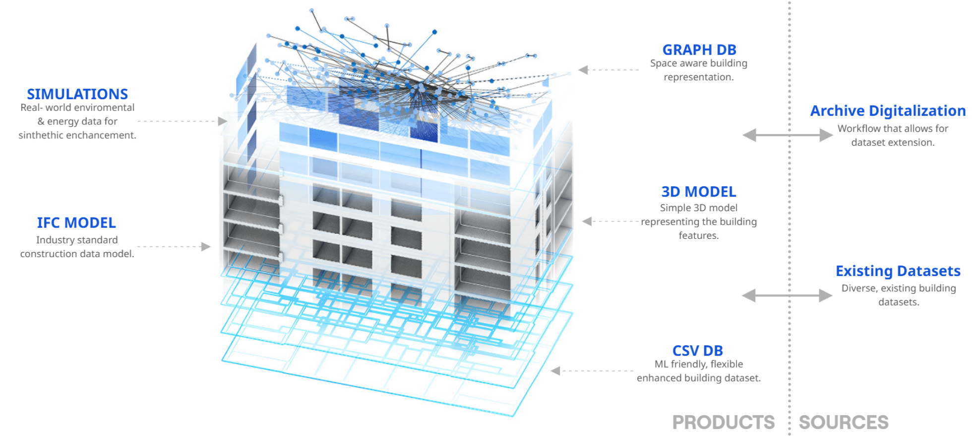
#03 PIPELINE
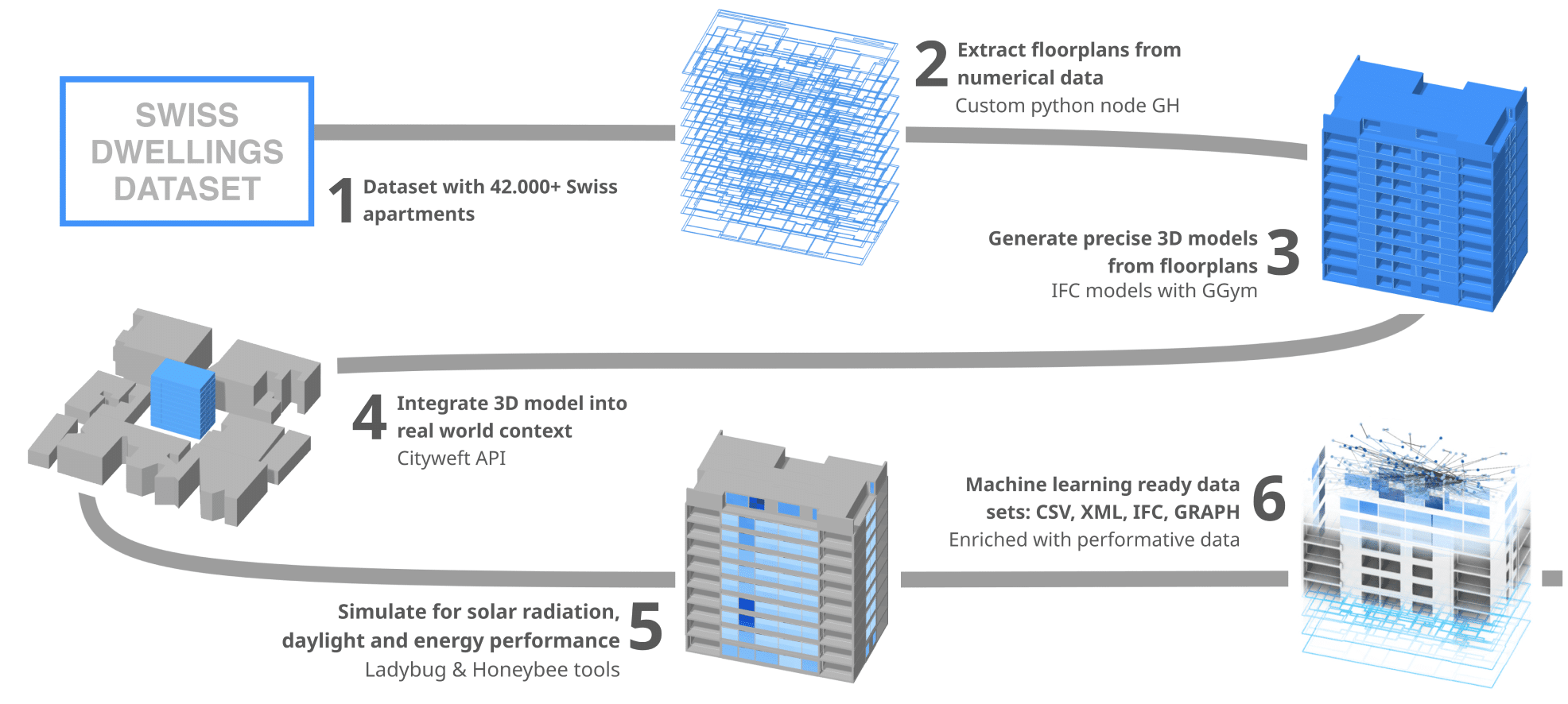
Our computational pipeline that turns the Swiss Dwellings CSVs into a simulation-enriched, multi-format dataset. We begin in Grasshopper, where we parse the relational tables (areas, openings, separators) into per-storey 3D reconstructions with consistent data-tree structures and stable IDs. Each building is then situated in a plausible urban context and mapped to an EPW climate file; with that scaffold we run Ladybug Tools simulations directly on the Grasshopper model—room grids and window proxies—using uniform tolerances.
The raw outputs are saved as normalized tables keyed by building_id / storey_id / space_id / window_id, ensuring every value is traceable to a unique element in the reconstruction. Once simulations are complete, we author the IFC using Geometry Gym and embed the results back onto the corresponding elements as custom properties. From this enriched IFC we compile two graph views in Python notebooks—space adjacency and circulation—using the same stable keys.
Then we export the full corpus in synchronized layers: IFC (semantics and topology), CSV/XLSX (per-room/per-window metrics and building summaries), and GraphML/pickle (networks for analysis). Throughout, deterministic identifiers, versioned snapshots, and small QA checks (counts, reachability, opening parity) make the pipeline reproducible, auditable, and ready for downstream analytics and ML.
SWISS DWELLINGS DATASET
Swiss Dwellings is a large, open dataset curated by Archilyse AG that aggregates real Swiss residential buildings. It provides tens of thousands of apartments across roughly three thousand buildings, released under CC-BY 4.0. The corpus is delivered as normalized CSV tables with geometry encoded in WKT: areas (rooms), separators (walls/railings), openings (windows/doors), and features (fixtures) in a consistent local site coordinate system. Each record is linked by stable keys (site_id, building_id, floor_id, unit_id, area_id) and accompanied by rich attributes—room category, net area, compactness, wheelchair navigability, counts of doors/windows, and other layout flags. For privacy, exact addresses are not provided; instead, location characteristics and ratings are offered at an abstracted level. This structure makes Swiss Dwellings an excellent source for deterministic reconstruction: tables join cleanly, geometry is explicit, and semantics are consistent enough to be re-used downstream.
SELECTION & CURATION
We chose Swiss Dwellings as the raw geometric and semantic backbone for our thesis dataset, but we did not consume any of its precomputed analysis layers. Instead, we rebuilt every building from the CSVs and generated our own synthetic simulation data on top of the Grasshopper reconstruction. Working directly from geometries.csv and the relational tables, we parse WKT into storey-organized room footprints, openings, and separators; normalize IDs and naming; and keep both residential and selected non-residential cases to widen typological coverage. Where the source omits values (e.g., vertical dimensions), we parameterize them explicitly in our reconstruction step rather than inferring from SD. We freeze a versioned snapshot of the dataset to guarantee repeatability, then route the rebuilt models into our context-assignment and EPW mapping to run daylight/solar analyses. Only after these synthetic simulations are produced do we author the IFC and embed results back as properties, preserving one-to-one correspondence through the same stable keys. The outcome is a curated, version-controlled pipeline that leverages Swiss Dwellings’ clean geometry and metadata while keeping all performance layers authored by us.
CSV EXTRACTION
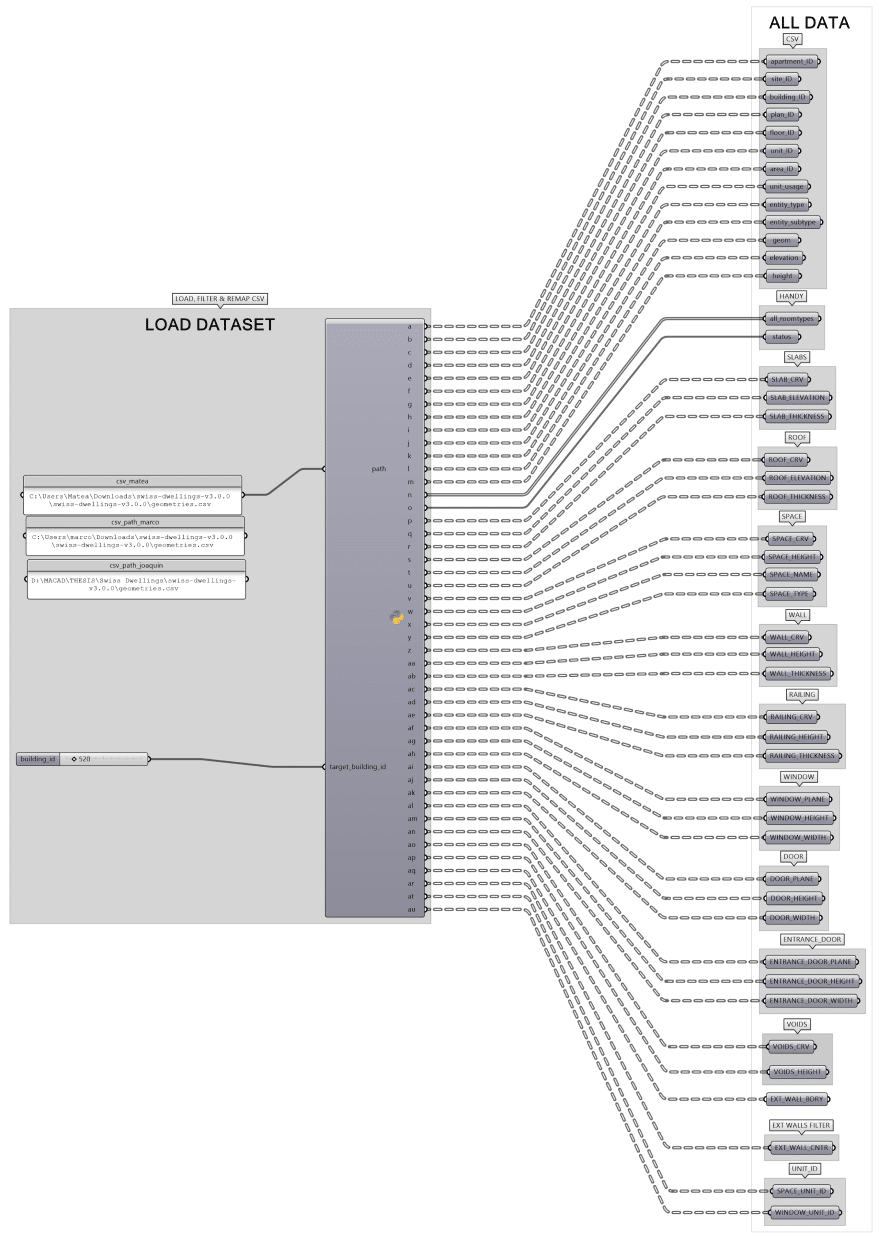
To retrieve and prepare data from the Swiss Dwellings dataset, we developed a custom Grasshopper Python component that reads the CSV files, extracts the required fields, restructures them, and outputs workflow-ready data. This step forms the foundation for all downstream tasks, including IFC authoring and simulation model generation.
More than two million records are first partitioned by building ID so that each building is processed independently. For every building, relevant entries are filtered, normalized, and reshaped into Grasshopper DataTrees—an essential structure for the workflow. The canonical path depth is:
{ building ; level ; element }
Where applicable, additional Python nodes introduce a residential-unit tier—handled separately because not all spaces are residential:
{ building ; level ; residential unit ; element }
Finally, numerical attributes are converted into geometry for IFC creation. For example, wall centerlines are derived from wall polygons and used directly as inputs for IFC wall objects.
CONTEXT INTEGRATION
Integrating urban context was a crucial step in our workflow, as it enabled us to place buildings within realistic surroundings and run environmental simulations that depend heavily on context. Since the dataset we used did not provide georeferenced locations, we designed a method to systematically assign each building to a suitable city and neighborhood. The process started by analyzing the bounding box and geometric characteristics of each building.
Parameters such as height, footprint size, overall shape, apartment area, number of levels, and apartment count were extracted. These features were then compared to the ranges defined in our city dictionary. Each building was matched to the top three candidate cities where its geometry most closely aligned with local housing typologies.
From these candidates, we selected one address to be processed through a custom Cityweft component developed in Grasshopper. The component used the Cityweft API to retrieve accurate urban meshes of the surrounding neighborhood, which could be directly imported into Grasshopper. This eliminated the need for manual context reconstruction and ensured consistency across different sites.
Once the context was imported, we compared the bounding box of the neighborhood with the building model to identify the best placement. In cases where adjacent structures would unrealistically block daylight or window façades, we selectively culled surrounding buildings to maintain a proper fit.
Along with the urban fabric, with the matched address and custom python components we provided EPW weather files required by Ladybug Tools for environmental simulations and city-specific U-values necessary for energy analysis. This integration ensured that both the geometric and climatic aspects of context were aligned.
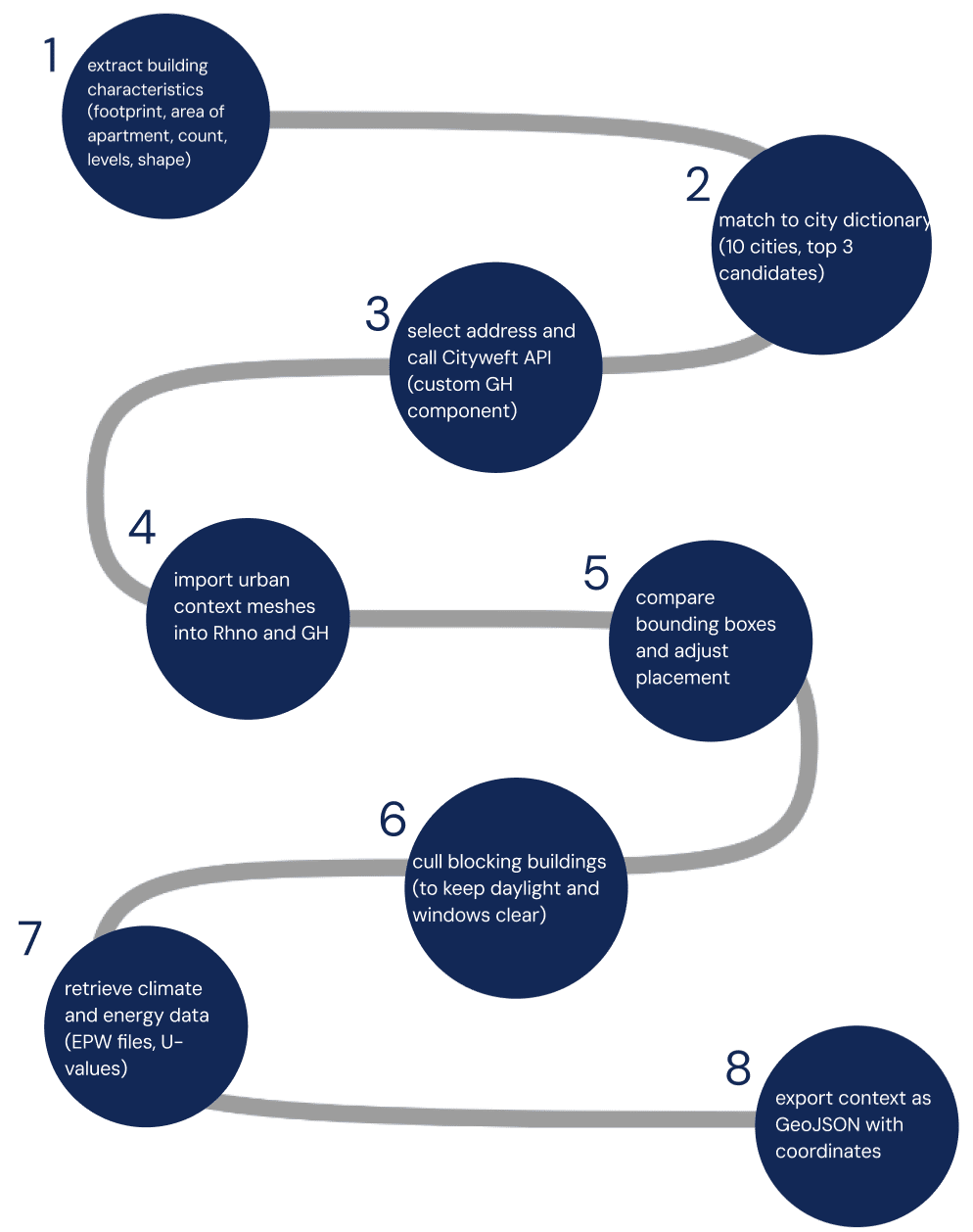
At the end of the process, the context was exported in GeoJSON format, with geographic coordinates directly extracted through the custom Cityweft component. This made the dataset not only suitable for performance simulation but also interoperable with GIS environments, allowing future extensions and broader usability. By combining geometric matching, contextual geometry, and climate-specific data, the workflow provided a robust framework for situating buildings into realistic, simulation-ready urban contexts.
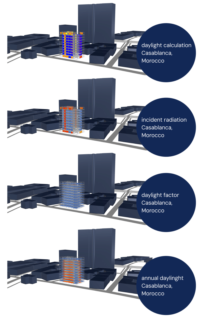
PERFORMANCE ANALYSIS
To evaluate the environmental performance of our buildings, we integrated Ladybug Tools into Grasshopper and developed a semi-automated workflow. A custom Python script was created to retrieve EPW weather files for each assigned city, ensuring that simulations used accurate, location-specific climate data.
Before simulations could run, we addressed geometry issues inherited from the original dataset. This step was essential, as inconsistencies in the floorplans—such as misaligned walls, overlapping elements, or incomplete boundaries—would otherwise prevent reliable results. Once geometry was cleaned, we prepared simulation-ready models for windows and rooms.
For windows, we calculated two main metrics:
- sun hours on the first day of each season (winter, spring, summer, autumn).
- incident radiation for the same periods.
These results were saved in CSV files, with one entry per window, creating a structured dataset for further analysis.
For rooms, we performed daylight simulations, including annual daylight availability, using custom sensor grids at 1-meter spacing. This provided a consistent and comparable basis across different layouts. As with windows, the results were exported and stored systematically for each room.
The simulation process required significant data preparation and was relatively slow due to the scale of the dataset, but it ensured high-quality results. Importantly, the outputs were not only saved externally but also embedded into the models themselves. Simulation results were added as custom properties to IFC elements, making them directly available for downstream workflows such as energy modeling or machine learning applications.
ENERGY SIMULATIONS
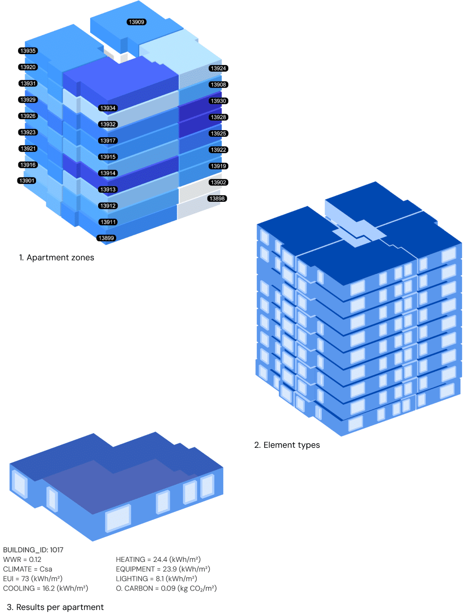
Additional performance data are obtained from annual energy-load simulations conducted in Honeybee at the apartment scale. Each unit is modeled as a self-contained thermal zone ), isolating residential spaces.
To prepare the models, the geometry is cleaned and partitioned so that space boundaries align with apartment perimeters. Boundary conditions are then assigned with the same adjacency workflow used earlier: exterior envelopes are set to outdoor, ground-contact elements to ground, and inter-apartment partitions to adiabatic (or explicitly linked to adjacent zones when required). This yields consistent heat-transfer paths and avoids double counting through shared walls.
Material properties, system archetypes, and orientation are inherited from the context placement. For each location, a predefined envelope set of U-values is applied. Weather files and design-day data are drawn from the selected climate, and each model runs an annual simulation with consistent timesteps and sizing routines.
Per-apartment outputs recorded include:
- Window-to-wall ratio
- Climate type
- EUI (kWh/m²)
- Cooling demand (kWh/m²)
- Heating demand (kWh/m²)
- Equipment demand (kWh/m²)
- Lighting demand (kWh/m²)
- Operational carbon (kg CO₂/m²), derived from end-use energy and location-specific emission factors.
IFC
An important part of our workflow was the creation of Industry Foundation Classes (IFC) Models.
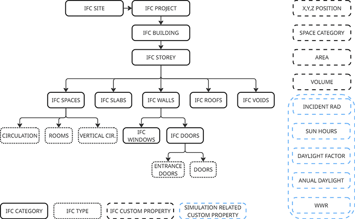
After reconstructing geometry from the Swiss tables, each building is authored as IFC2x3 so topology and semantics survive across tools. We keep the full spatial tree—Project → Site → Building → Storey—and place all elements under the correct storey so elevations and containment are explicit. Openings and host relations are written as true IFC relationships (host wall → opening → filled by door/window), which is crucial for downstream reasoning and counts. The result is not only viewable but queryable: every wall, slab, space, door and window can be recovered with its container storey, its hosts, and its footprint/volume for quantities or graph extraction.
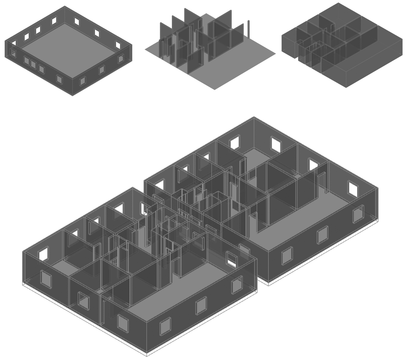
The Grasshopper definition loads cleaned per-storey inputs (space outlines + heights, wall centerlines + thickness, and door/window axes + sizes), normalizes lists/trees, and feeds ggIFC components in four passes:
- Spatial scaffold. Project/Site/Building/Storeys are created first; storey elevations come from the dataset; element placements are defined in the storey frames.
- Spaces & slabs. Space footprints are extruded to their storey heights and exported as IfcSpace; floor plates are built from the same outlines as IfcSlab so areas/volumes line up.
- Walls. Wall centerlines and thickness drive prismatic wall geometry; these are exported as IfcWall (StandardCase where applicable) with the correct storey containment. External/internal flags and thickness come from the filters you run upstream in the script.
- Openings, doors, windows. Door/window axes and nominal sizes generate IfcOpeningElement cuts in the target walls; those openings are then filled by the corresponding IfcDoor/IfcWindow instances. That sequence guarantees clean host–opening–filling chains rather than boolean-only geometry.
Across these passes the graph shows small QA blocks (counts per storey, preview panels) to verify that element totals, opening counts, and list lengths match the source tables before writing the file.
Another layer of improvement was to enhance the IFC models with a series of custom props. To achieve this, we created a series of Property Sets that enrich the model with additional layers of data not present in the original db.
Every element carries a location triplet (centroid X/Y/Z in meters) and a set of keys (building/storey/space/unit identifiers) so the IFC can be merged reliably with your CSV tables and graph exports without geometric matching. Spaces include their semantic room type, net area and height; walls and slabs include thickness/height where available; doors/windows keep their nominal sizes. We reserve fields for simulation results (e.g., daylight/solar summaries at space or façade level) so performance data can live on the exact elements it describes and be queried directly from IFC later.
The use of Custom Properties opens the possibility for database enhancement in the future, being our direct next steps to enhance our models with Energy Simulation data.
GRAPHS
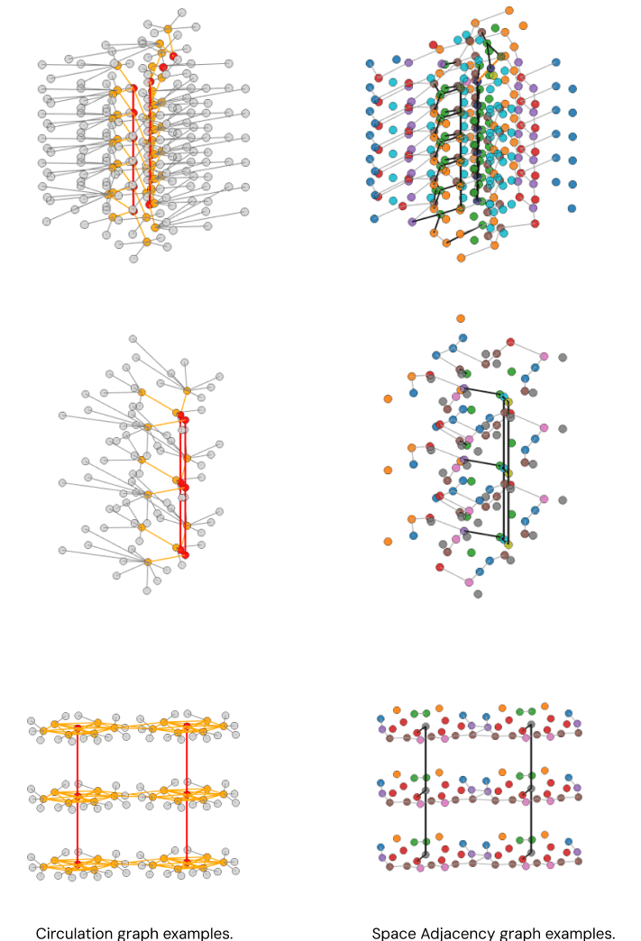
We model each building as graphs because they preserve the semantics and spatial logic that get lost in raw geometry. Nodes are primarily spaces (from the IFC) with attributes carried over from the model—type, net area/height, storey, unit keys, and centroids—so they can be joined to tables or simulations without guesswork. From those nodes we derive two complementary views. The space-adjacency graph encodes where spaces touch: edges are created when two spaces share a boundary above a small overlap threshold or when an opening connects them, and we record basic geometric metadata (shared length, contact type). The circulation graph captures traversable connections only: edges appear where movement is possible through doors, corridor connections, or vertical links such as stairs; we keep door or opening descriptors and the storey change when present. Keeping both views lets us run standard network measures (reachability, shortest paths, centralities, communities) and compare “physical adjacency” against “actual walkable paths,” which is essential for wayfinding, egress, program clustering, and ML feature extraction on building topology.
Our notebooks take the authored IFC as the single source of truth and compile graphs in a deterministic sequence.
First, we parse storeys, spaces, walls, doors, and window placements, normalize identifiers, and compute centroids so every node has stable keys and coordinates.
Next, we generate adjacency edges by intersecting space boundaries and by linking spaces that meet across an opening; tolerance and minimum-overlap rules come from the dataset scale so false contacts are filtered out. We then specialize these edges into the circulation layer by keeping only walkable connections (doors, corridor–corridor continuity, and inter-storey links for stairs/landings). Each edge carries lightweight attributes needed later for weighting or filtering (e.g., edge type, shared length or door nominal size when available, and storey for vertical links).
Finally, we export the graphs in CSV tables (nodes/edges), GraphML for interoperability, and a pickle/NetworkX snapshot for fast analysis, alongside simple QA reports that flag isolated spaces, unreachable components, and count mismatches between adjacency and circulation. The result is a pair of building graphs that are reproducible, queryable, and ready to cross-reference with your performance data and learning tasks.
#04 ENHANCED DATASET
This chapter presents the Enhanced Dataset—the finalized, machine-ready corpus that synchronizes geometry, context, and performance across three layers. Starting from Swiss Dwellings CSVs, we reconstruct each building in Grasshopper, run daylight and solar simulations on that model, and write normalized CSV/XLSX tables keyed by stable IDs (building_id, storey_id, space_id, window_id).
We then author one IFC2x3 per building with Geometry Gym, embedding the same results as lightweight property sets, and derive space-adjacency and circulation graphs from that enriched IFC. The chapter summarizes what each layer contains, how the IDs align for lossless joins, and the basic QA that keeps the bundle reproducible and queryable for analysis, ML, and downstream design tools.
CSV
We export three CSV tables for fast analysis and ML:
- Windows_simulation (per-window incident radiation and seasonal sun-hours, with window geometry fields),
- Rooms_simulation (per-room daylight metrics such as daylight factor and annual daylight, with space type and unit keys),
- building_info (project-level summaries like apartment count, average apartment area, levels count, EPW id/address).
Every row is keyed by simulation_id, building_id and the relevant element id (window_id or space_id), so joins with our graphs and IFC are one-line operations. CSV is ideal for notebooks and pipelines (pandas/Polars/R/SQL), version-control diffs, bulk processing, and quick feature engineering.
XLSX/XML
We also provide a single XLSX/XML package with three tabs/sections that mirror the CSVs. XLSX is optimized for human QA, stakeholder review, and lightweight BI dashboards.
The matching XML exposes the same schema in a strict, hierarchical, machine-readable format, making it easy to validate, ingest into relational databases, and query with standard tools (e.g., XPath/XQuery). Using the same stable keys (building_id, storey_id, space_id, window_id) across CSV/XLSX/XML guarantees lossless round-trips and straightforward enterprise ETL and app integrations.
IFC
As part of our enhanced dataset, we create one IFC2x3 file per building, authored in Grasshopper with Geometry Gym, as the interoperable “snapshot” of the final dataset.
Each file encodes the full spatial scaffold—Project → Site → Building → Storeys—with instances for Spaces, Slabs, Walls, Windows, Doors (and Roofs/Void cuts where present), all placed in the correct storey frames. Openings are written explicitly (wall → opening → filled by door/window), so host relations, counts, and quantities are recoverable without geometry heuristics. To keep the IFC synchronized with the rest of the corpus, every element carries compact custom
Property Sets: stable keys (building/storey/unit/space/element IDs) and centroid X-Y-Z for joins, plus our simulation summaries on rooms and windows (e.g., daylight/solar metrics and WWR). The result is a self-contained, queryable model that opens in standard BIM viewers and analysis toolchains, and that lines up one-to-one with our CSV tables and graphs for downstream analytics and ML.
GRAPHS
Here we export each building’s topology as a portable graph bundle that’s ready for analysis and ML: compact CSV tables (master_nodes, master_edges, buildings_metadata) for feature engineering; GraphML for interoperability; a fast pickle snapshot for Python/NetworkX; JSON analytics with per-building metrics; and lightweight HTML/PNG views for human inspection. Together these formats make the same, ID-stable graph usable in notebooks, pipelines, and future apps—whether you’re training a GNN to learn circulation patterns, running community detection for program clustering, or benchmarking accessibility and egress. Treating buildings as graphs aligns architectural data with the relational inductive biases leveraged by modern graph networks [1], paving the way for next-gen software where the “building kernel” is a topology-aware graph rather than a loose CAD model.
#05 CONCLUSIONS AND FUTURE WORKS
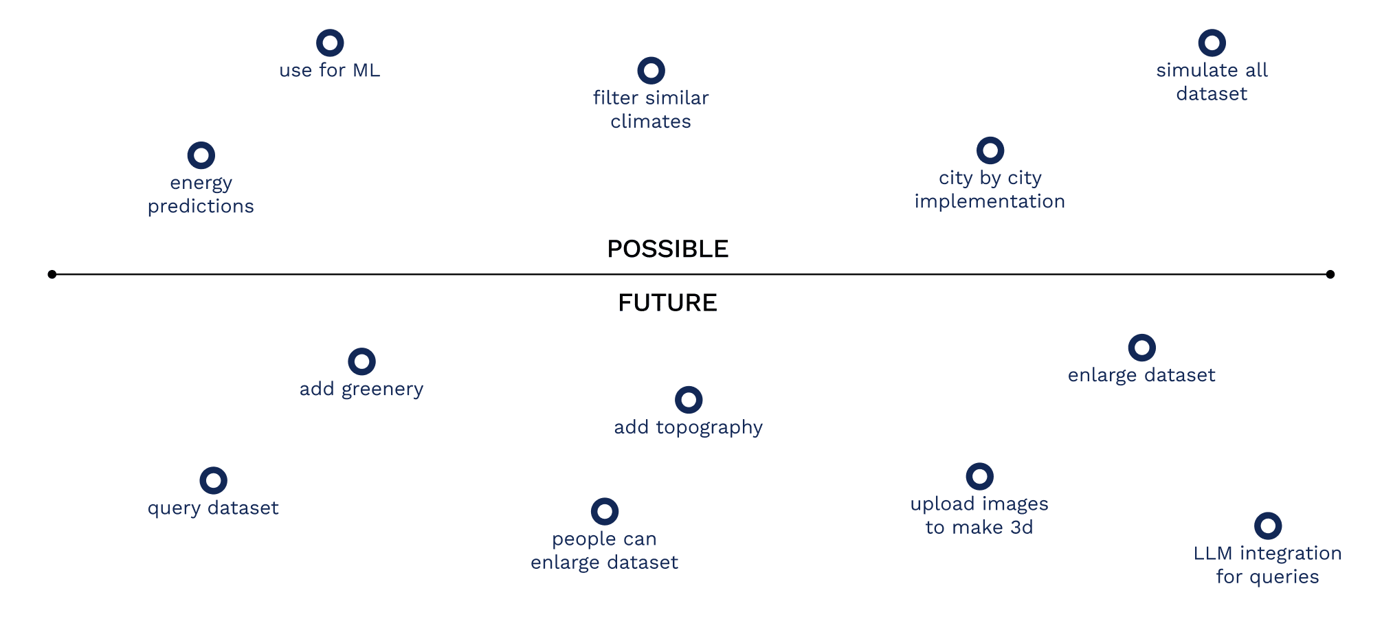
Here we distill the project’s state and outline what comes next. We proved that Swiss Dwellings CSVs can be rebuilt into a coherent, simulation-enriched corpus—reconstructed in Grasshopper, exported as synchronized CSV/XLSX, IFC, and graphs—and we ran daylight/solar analyses at scale with stable IDs across layers. The main gaps are operational rather than conceptual:
batch robustness, explicit graph relationships, cloud-based energy simulations, and richer context (topography/greenery). The near term focuses on scaling coverage, tightening QA and exports, and publishing a versioned, queryable release; the medium term adds LLM-assisted querying and community contributions via an open site.
DIAGNOSTICS
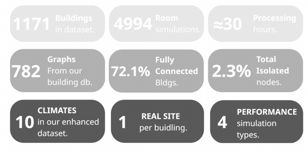
As of this booklet the corpus is partially built and validated. We’ve reconstructed and simulated 1,171 buildings, producing 4,994 room-level simulations across 10 climates, with one real site per building and four performance simulation types. End-to-end processing for the verified subset took about ≈30 hours. From these runs we compiled 782 building graphs; 72.1% are fully connected and only 2.3% of nodes are isolated—useful baselines for connectivity and data quality going forward.
The gaps are known and tractable. Some buildings failed during batch runs (geometry/ID edge cases) and a portion of IFC exports didn’t validate, which is why not every processed building yielded a clean graph. The current graph builder still infers relationships; moving to an explicit relationship layer (door↔space, space↔space, vertical links serialized during reconstruction) will harden graph creation and improve coverage. Energy models are issued, but full energy simulations are still queued for cloud execution. Together, these diagnostics frame the work as a solid spine with clear next steps: stabilize batch reliability, make relationships explicit, finish the cloud energy pass, and then scale beyond the present snapshot.
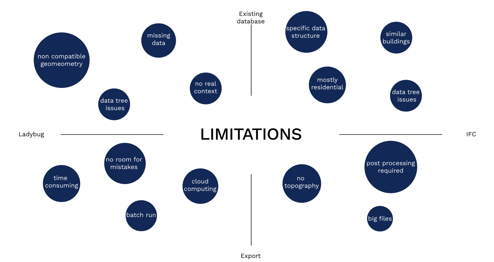
LIMITATIONS
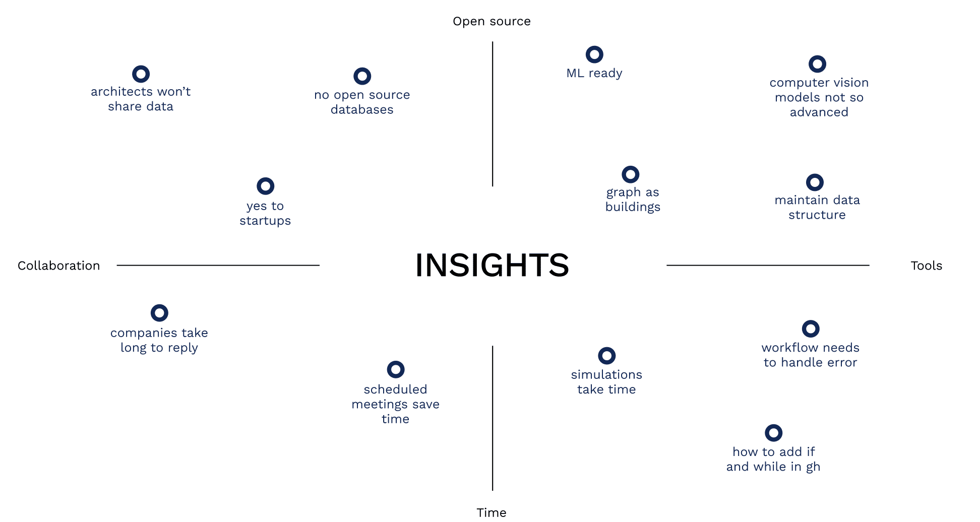
INSIGHTS
CONCLUSIONS
This thesis project aimed to answer the following question:
How can we create a workflow to enrich existing floorplan databases with performative data?
Results show that architectural CSVs can be rebuilt into a coherent, simulation-enriched corpus that is consistent across different output formats. The strongest result is methodological: stable identifiers and disciplined DataTree handling let us trace every metric back to a unique element and keep exports in lock-step.
Along the way we hit the real pain points of the field: patchy or missing inputs, the absence of real-world context in source datasets, and the brittleness of Grasshopper data trees when scaling to complex hierarchies. Performance simulations are accurate but computationally heavy, making geometry QA (open loops, overlaps, orphaned elements) and caching indispensable. On the packaging side, IFC files grow quickly and become unwieldy without strict scoping, and the lack of topography further limits contextual fidelity.
Beyond pure tech, structural barriers remain: architects are often reluctant to share data, truly open architectural corpora are rare, and many computer-vision tools for parsing plans or BIM are still early-stage—keeping pipelines depending on its current foundation: a clean, well-organized, consistently labeled dataset is essential—and, in practice, the hardest asset to obtain.
OUTLOOK
The path forward is clear and practical. Upstream, add a pre-ingest validator and schema map for the source CSVs, automatic context assignment (city + EPW + optional terrain), and guardrails for GH data-trees (typed branches, shape checks, and unit tests) so batch runs fail fast. For simulation scale, combine geometry cleaning with cloud batching, result caching, and—where appropriate—surrogate models to cut runtimes. For packaging, keep IFC lean (typed subsets, deterministic GUIDs, compressed deliverables) and push heavy analytics to the tabular/graph layers; add terrain/topography as an optional context layer. On the ecosystem side, publish versioned snapshots with manifests and QA reports to encourage reuse; design contribution guidelines that protect privacy while enabling openness; and keep investing in graph-native representations so adjacency, circulation, and performance can be learned directly by ML. In short, the workflow is viable and reproducible today; by hardening data handling, scaling simulations responsibly, and embracing open, graph-centric exports, this line of work can seed the next generation of performance-informed architectural tools.
PROGNOSTICS
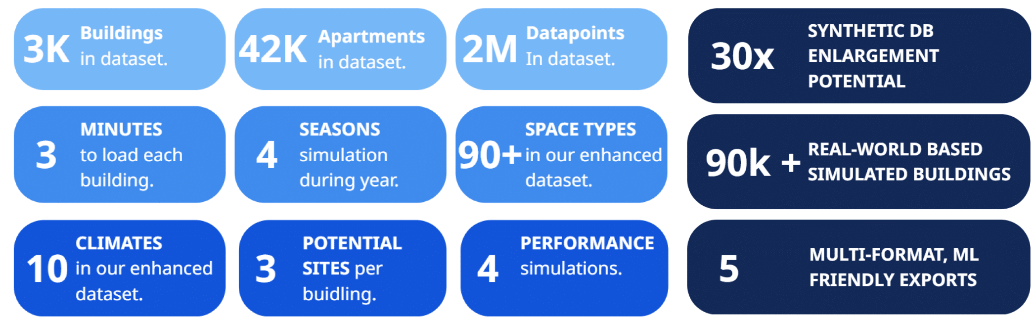
The current dataset forms a strong foundation, but it also highlights the potential for further growth and refinement. The original Swiss Dwellings datset, includes around 3,000 buildings, 42 apartment typologies, more than 2 million datapoints, and over 90 space types.
From the total buildings, around a 30% was processed through the pipeline.
Each building takes approximately three minutes to load, which makes the process computationally demanding but still manageable for large-scale exploration. For every building, we already run four different environmental simulations (sun hours, radiation, daylight, and annual daylight) across four seasonal days in ten different climates. To account for variability and reduce bias, each building can be matched to up to three candidate cities/climates, which provides both flexibility and robustness in analysis.
Looking forward, the dataset can be broadened in several directions. A direct next step would be to apply all three climate matches per building, effectively multiplying the dataset’s size and relevance without additional architectural modeling. This would make it possible to study how identical geometries perform across different contexts and climates, offering valuable insight for predictive models. On the technical side, the dataset can be distributed in five machine learning–friendly formats: CSV, XLSX, XML, IFC, and Pickle, ensuring compatibility with a wide range of analytical and computational pipelines.
In the longer term, further expansion could include additional building samples, more contextual data layers such as topography or greenery, and integration of real-world measurements to complement simulated values. By broadening the dataset in this way, we move closer to creating a comprehensive, flexible, and open architectural resource that supports both scientific research and design innovation.
POTENTIALS
REFERENCES