
Context
Is additive manufacturing going to change the way we fabricate?
Certainly it is, additive manufacturing has an immense growth potential with a 22% annual growth as it has offers mass customization and reduced waste. One of the challenges in additive manufacturing is to improve the precision and reliability of the manufacturing process. This can be done by sensing and optimization using enhanced software’s which itself will be a 43.5 Billion market by 2028.
What are the problems prevailing in the industry?
Synchronization of digital and physical world is a big problem in robotic fabrication. Also, it is time consuming to fix multiple problems at the same time, so it would be better if we can predict some of them in advance. Prototyping takes the most amount of time in additive manufacturing which makes it more expensive and less efficient.
How can we fix these problems?
Having a feedback loop in the manufacturing workflow can enhance quality and save time. This technology demands adaptable workflows. Also, neural networks are perfectly suited to understand complex parameters to address problems like shrinkage
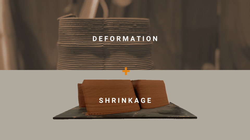
D E F O R M A T I O N + S H R I N K A G E
Despite clear economic and environmental benefits, manufacturers have difficulty implementing additive manufacturing at scale. This is due to concerns about its dimensional accuracy and structural integrity. One of the shortcomings of additive manufacturing across all materials is that, it shows deformation due to gravity and shrinkage after curing process which is very difficult to control and overcome. I am focusing on clay as a material for 3d printing to evaluate my research as it shows significant deformations after printing and its ease of prototyping. Nowadays it is being explored extensively for its utility in 3D printing due to its sustainability and adaptability for mass customization.
Research Goal
In the potentially growing demand for 3D printed highly customized mass produced elements, an adaptive workflow to predict and correct deformations can provide a cost-effective means of digital fabrication with enhanced dimensional accuracy. This research aims to bridge the gap between digital model and physical results of 3d printing by utilizing data acquired during the prototyping phase to train an artificial neural network capable of simulating deformations and correct it by G-code optimization.
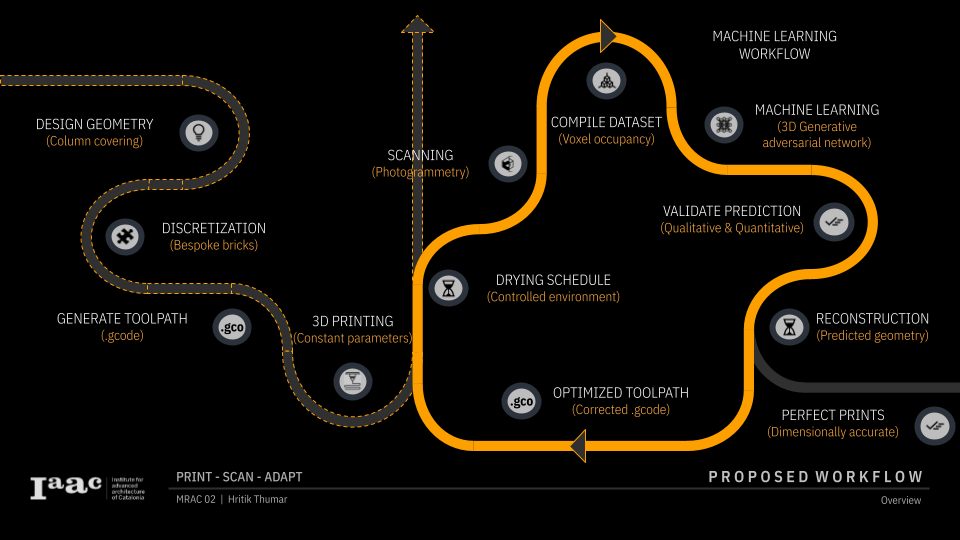
Adaptive workflow
The entire workflow is broken into ten separate parts. The first five steps represent the industry standard workflow for any 3D printing process. It begins with design, then discretization to make it printable, producing toolpath, printing, and finally postprocessing. Using machine learning, I’m adding an extra loop of processes to optimize printers for dimensional accuracy. We’ll go through each stage in detail.
Design Geometry
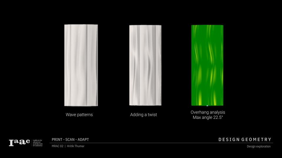
With the introduction of parametric design, the building industry is shifting from mass production to mass customization. To validate my research, I am creating a 3D printed column cladding system.So my goal is to use a machine learning approach to build a column cladding from bespoke 3D printed clay bricks, resulting in a flawless fit and finish. The patterns created by a moderate breeze on a curtain served as inspiration for my design. The column was created with wavy patterns that convey a sense of fluidity and lightness in space. After applying the surface texture, a twist is applied to expand the possibilities of 3D printing. Then, ensure that a 3D printable overhang analysis is performed.
Discretization
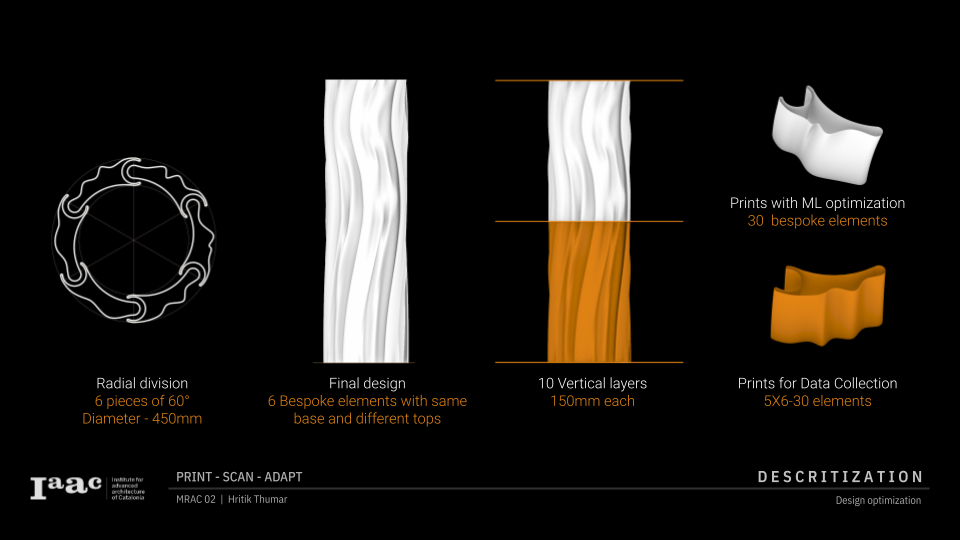
The column is broken into six pieces each layer. Then, to create a prototype, six sides were designed with the same pattern in the base and a bespoke design on top. The first five layers were printed to gather data for machine learning. The top five layers were printed using ml optimization.
The next step is to transform discretized geometry into a toolpath, which will generate a Gcode file for printing. The Gcode is then delivered to the 3D printer.
3D printing
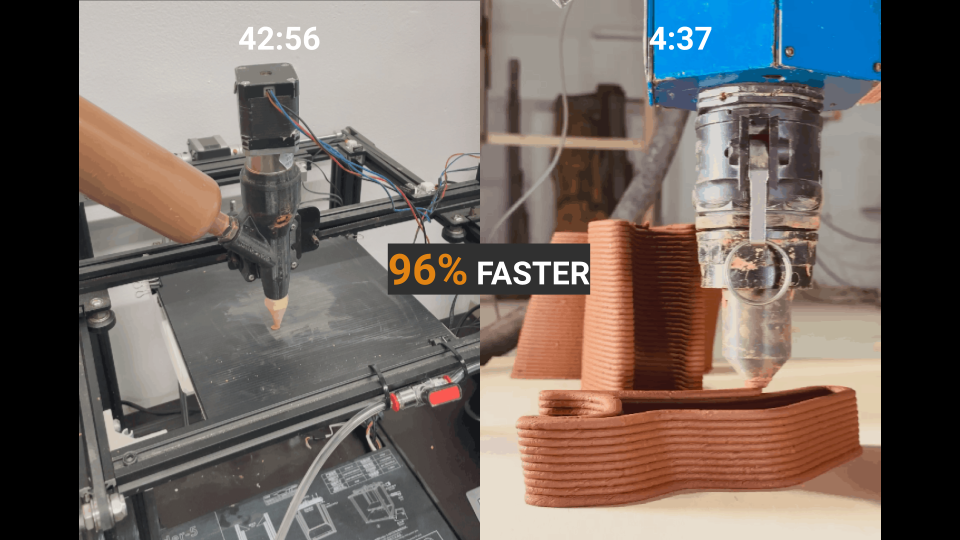
For printing, I tried two different scales. For initial testing, an ender cartesian printer was chosen because it is simple to set up. For the final prototype, a 6-axis robot with a continuous feeding mechanism was used. Ender takes 42 minutes to print each piece, whereas I can do the same in just over 4 minutes with the robot, making the operation 96% faster.
Scanning
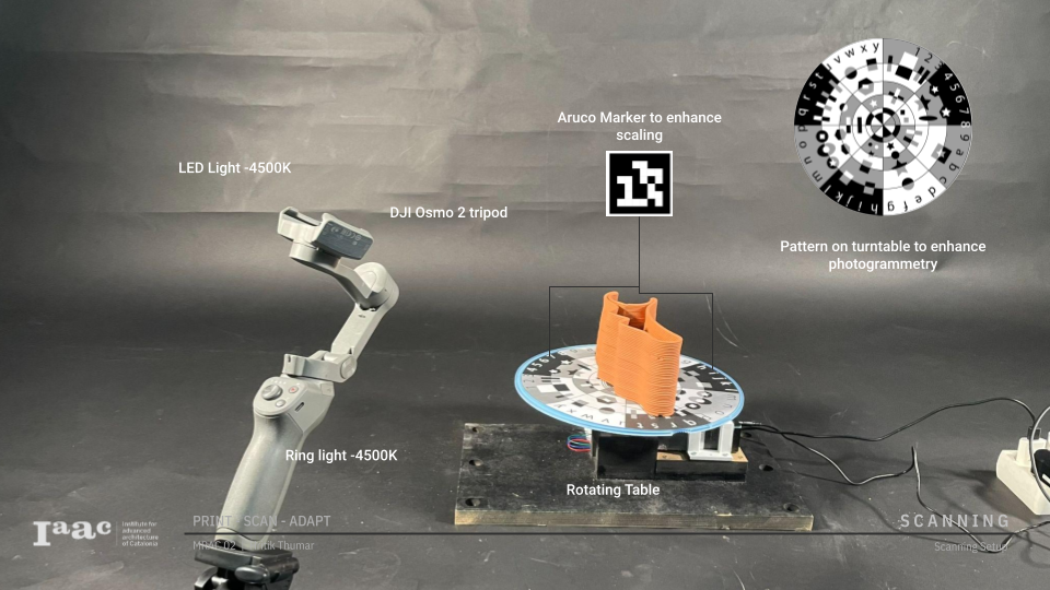
I automated my scanning setup by using a turntable and a tripod with pre-set angles. Then I improved the findings by adding patterns to the turntable, which dramatically boosted accuracy and reduced the amount of raw photos needed for a successful result. In addition, aruco markers were employed to pinpoint and scale rhino. All of these strategies resulted in precise scans every time, reducing scanning time by 60% to 2.5 minutes per scan.
Compiling Dataset
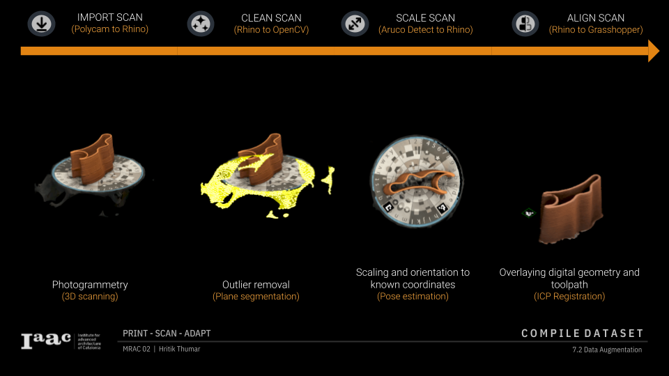
First, the scans are loaded into rhino. The scans are then cleaned up using opencv to remove any undesirable outliers via plane segmentation. These cleaned images are then scaled as needed and localized to known coordinates in rhino using aruco markers. Following localization, these scans are overlaid with digital geometry and toolpath, forming a foundation for generating various sorts of databases.
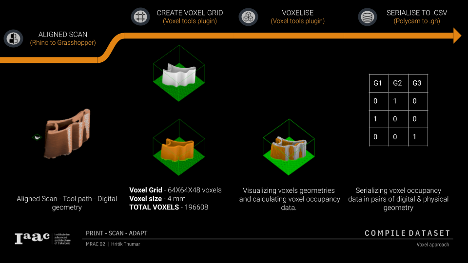
A plugin in grasshopper generates a voxel grid. I am using a 64x64x48 voxel grid. And I’m using a 4mm voxel dimension because it’s half of my print width. These geometries are subsequently voxelised, and the occupancy data is stored as boolean values. These values are then serialized as.csv files for ML.
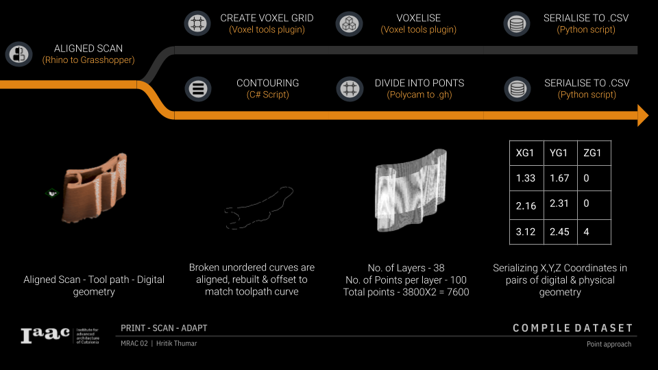
The scans for the points approach are contoured, aligned, reconstructed, and offsetted to match the tool path curve using a C Sharp script. These curves are segmented into points at predetermined positions. Each layer contains 100 points. The X, Y, and Z coordinates of these points are then serialized as pairs of digital and physical geometry in.csv format for ml. Because 30 geometries are insufficient for ml, the dataset is multiplied by mirroring geometries along all three axes using the numpy module in Python. So, in total, a dataset of 240 geometries was generated for ML.
Machine learning
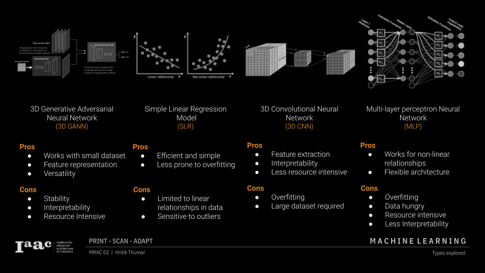
I tried four different ml methods for this application. Each has merits and cons. 3D GANN performs well on tiny datasets, however because it is generative AI, it only understands shape transformation. Linear regression is efficient and easy, but it only works with data that has linear connections. 3D CNN is ideal for understanding the correlation of movement between each point, but it requires a large dataset. MLP works well for this, although it is tough to learn and requires a larger dataset to begin with. Out of all of these, I’m going to discuss these two and compare their results.
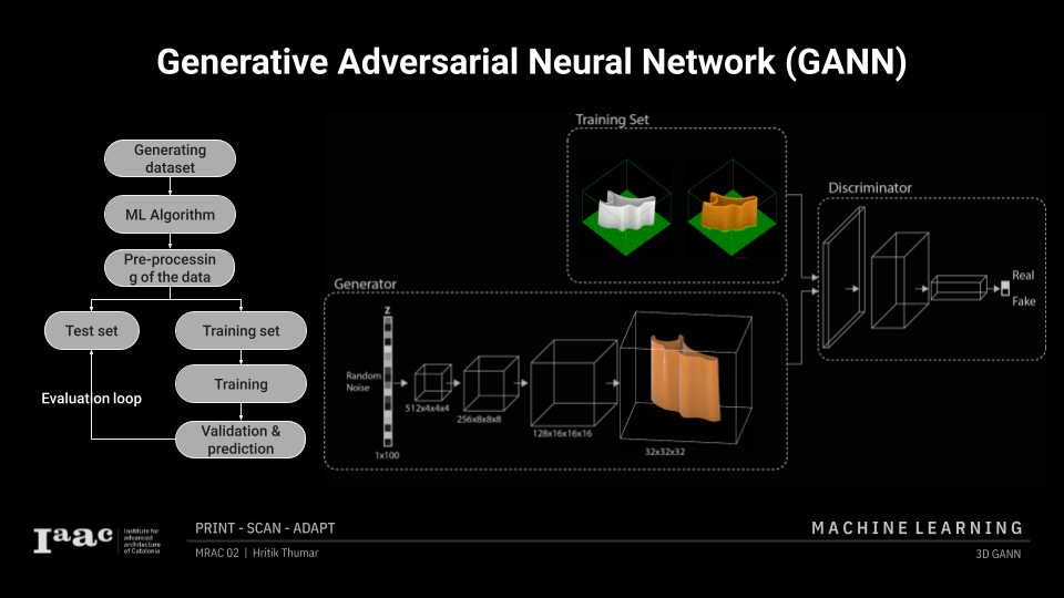
Here is a flowchart showing the entire machine learning workflow.
GANs are made up of two neural networks, a generator and a discriminator, which are trained simultaneously. The generator produces synthetic data, whereas the discriminator attempts to extract genuine samples from training data mixed with synthetic data. The discriminator offers input to the generator, which modifies its weights to improve the quality of the generated data. The discriminator also adapts to changes made by the generator, increasing its ability to distinguish between real and synthetic data. This cycle is repeated until the generator and discriminator have improved their performance.
GANs are great at creating synthetic data that closely mimics real data. This is beneficial in situations where gathering big volumes of real data is difficult or costly.
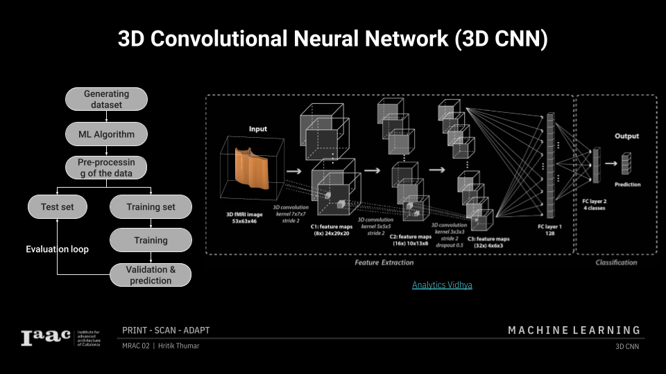
A 3D CNN processes volumetric data by applying three-dimensional filters over the input to extract spatial features, and then utilizing successive convolutional and pooling layers to gradually lower data dimensions while increasing depth. These layers are then enlarged to achieve the desired result.
Validate prediction
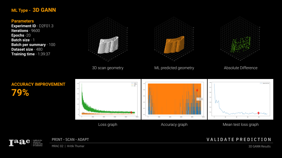
Here are the findings of the best-rained 3D GANN model. To visualize the findings, I use the plotly module in Python. I compare the 3D scan geometry of a known input object to the expected output of the algorithm; the absolute difference is shown in green dots. Because graphs are difficult to grasp, this strategy allowed me to better assess my training. This technique has a 79% accuracy rate.
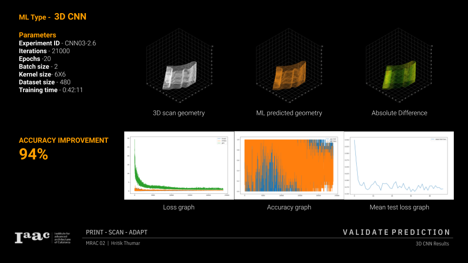
This is the best trained model for the 3D CNN model. As you can see, the absolute difference between the input geometry and the anticipated geometry is quite small. This model has a theoretical prediction accuracy of 94% for deformation.
Geometry reconstruction
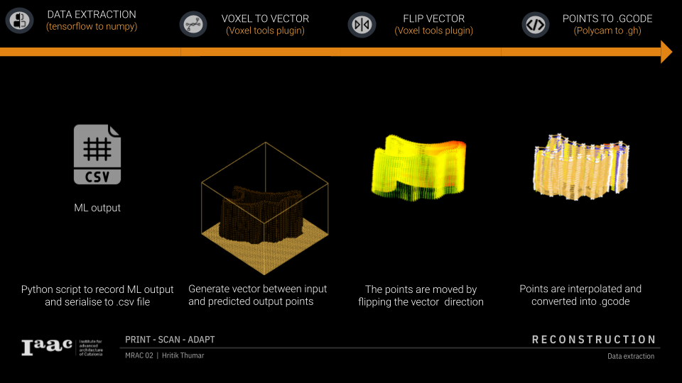
Using a Python script, ML learning output is recorded and serialized into.csv files. This is then recreated in grasshopper, and a vector representing the input and output points is formed. The vectors are then flipped, and new points are created. These points are then interpolated to form the toolpath.
This is optimized .Gcode is delivered to the robot, which prints it. This workflow loop continues to iterate until you achieve the necessary dimensionally correct prints.
Results
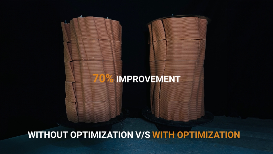
These prints are then combined and attached with threaded rods to the base. The end product demonstrates the workflow’s efficacy. On the left are the gaps caused by shrinkage and distortion. On the right, you can observe a roughly 70% improvement in fit and quality.
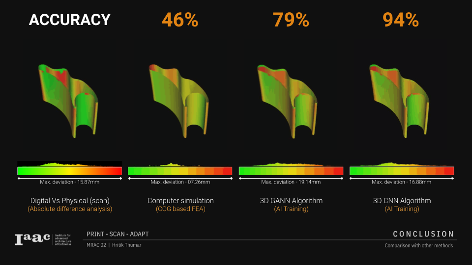
In conclusion, I examined the outcomes of three alternative ways to predicting shrinkage and deformation. The first one compares digital and physical geometries. It had a maximum deviation of 16mm. Then I performed a very rudimentary center of gravity-based shrinkage simulation, which yielded an accuracy of 46%. Then, 3d gann had a deviation of 19 mm, making it 79% accurate, while 3d cnn had a maximum departure of 17 mm, making it the most accurate method of prediction.
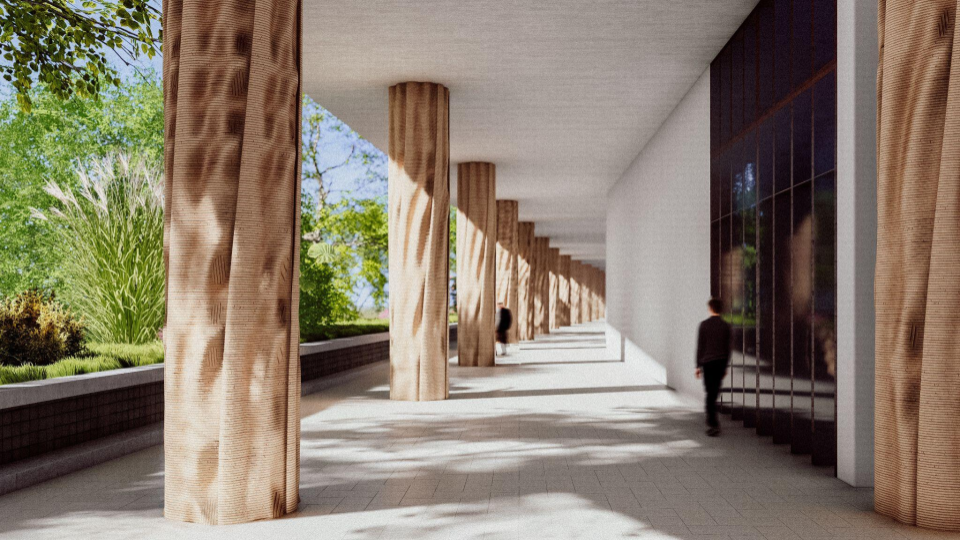
We can utilize 3D printed bespoke ceramic bricks as a lost formwork and pour concrete straight into it. It can also be used to conceal utilities and insulate any surface due to its natural qualities.
Limitations
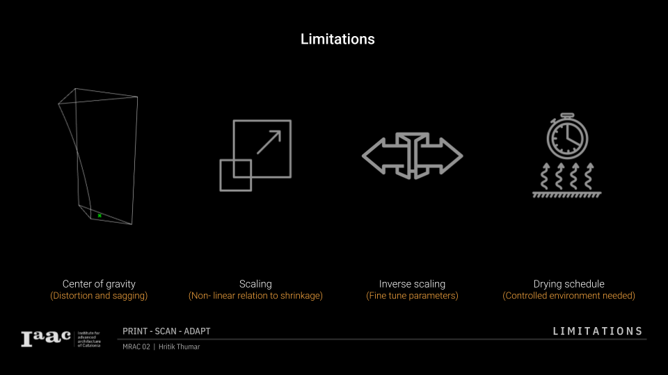
There are certain limits to this method. Centre of gravity analysis is critical when designing a part; otherwise, the prints droop with gravity, making my assembly process unfeasible without post processing. This method only works on specified scales. So, using the same model, you cannot forecast the shrinking of larger or smaller items. I’m inversely scaling the gcode to optimise it, however shrinkage is nonlinear, so this step can be optimised. A regulated environment is required to ensure even drying conditions.
Future steps
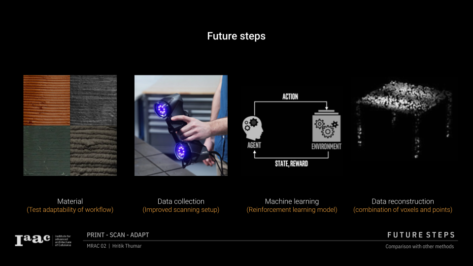
This method can be used to any 3D printing material. Structured light scanning can help improve data collecting. A reinforcement learning model can be used to generate a self-learning loop, leading to a generalized model for predicting deformation at any scale and with any material. The combination of points and voxels can be used to improve the reliability of data reconstruction.
