In this course we learned about the Robotic Operating System (ROS) and the MoveIt motion planning using Python for controlling robots. We also utilized development tools such as Git and Docker for managing the data. We learned about different types of sensors which helped for the robot’s motion visualization and scanning for the purpose of the project.
The goal of the course was to use the robot for scanning a 3d printed and post-processed block and compare it with the 3d digital model in order to acknowledge its real transformation due to shrinkage. We utilized the UR robot with a D405 Camera for the scan and afterwards we used Open3D (an open-source library that supports rapid development of software that deals with 3D data) for comparing the digital and the scan models.
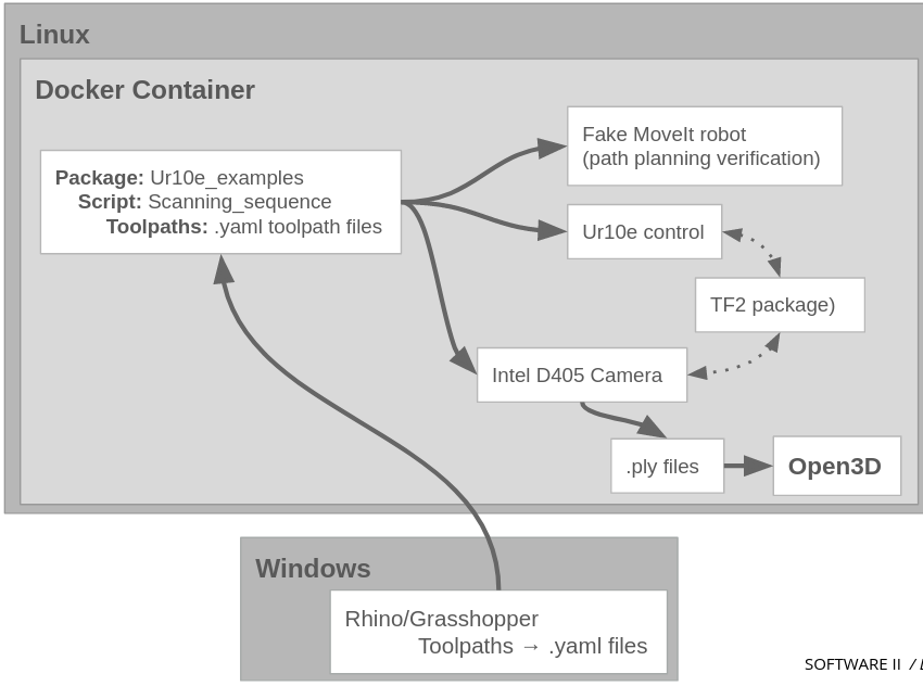
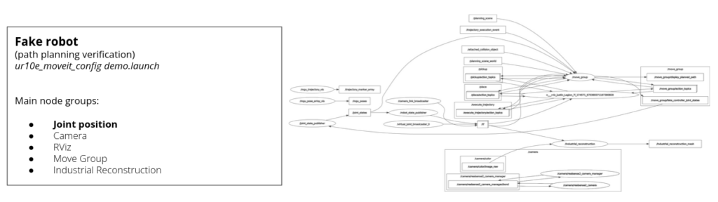
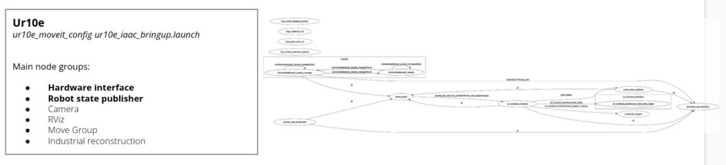
For the process, we defined an environment and a workspace with workflow shown below. First we created a digital environment to run the simulation and afterwards we made the real scan with the UR robot.
Motion planning
The robot uses motion planning for its movement in a given path or direction. They are condensed in two categories: free space planners and process planners. For this task, we used a process planner called PILZ motion, which has no requirement for obstacle avoidance given to a controlled environment and because it smooths speed while doing the scan.
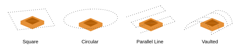
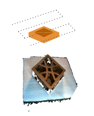
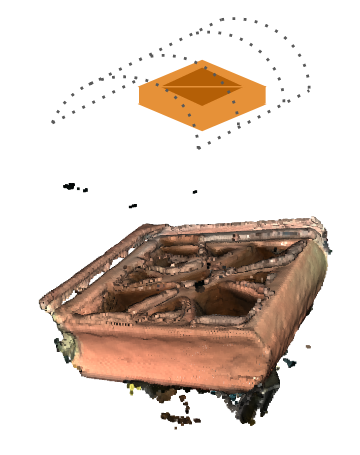
For better results, we generated 4 different tool paths which the robot would follow in order to record and scan the piece.
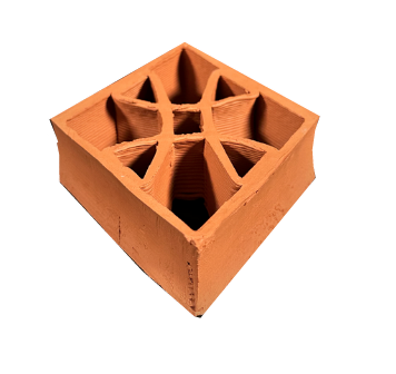
This is the piece which we decided to scan in order to compare the printed vs the digital model. Following up we will see the motion tool paths for the robotic UR scanning.
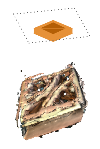
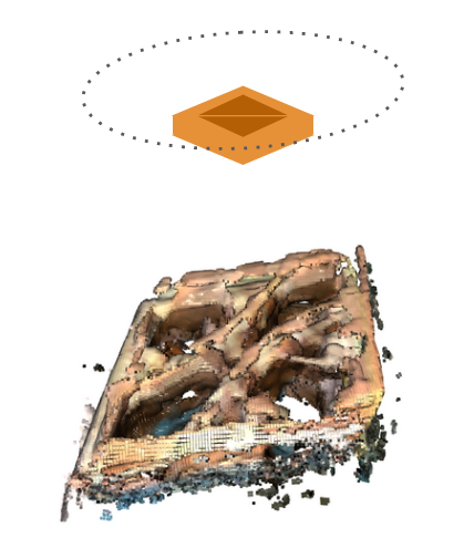
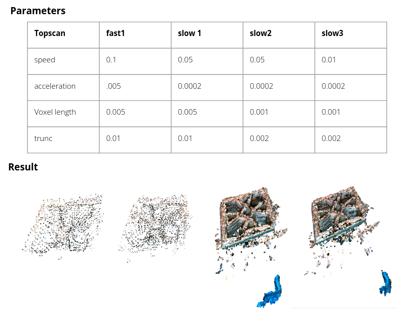
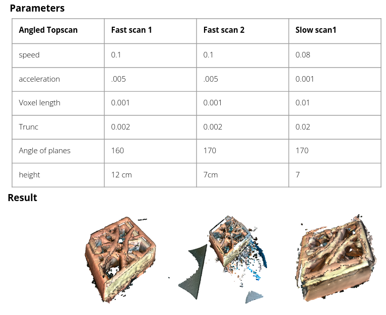
For these past scans, we identified different parameters like speed, plane angle, distance from the piece… which affect the result of the scan depending on their variations. The results from the different parameters with the point clouds are shown in the next images:
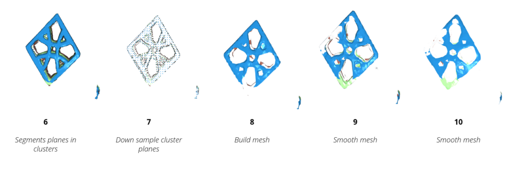
PCD Processing (Point Cloud)
After doing the scans, we selected the one that included the most real form compared to the real piece in order to start processing the point cloud scan. In class, we saw a tutorial which allowed us to control the point cloud following 10 different steps which could be useful for the final objective of the project.
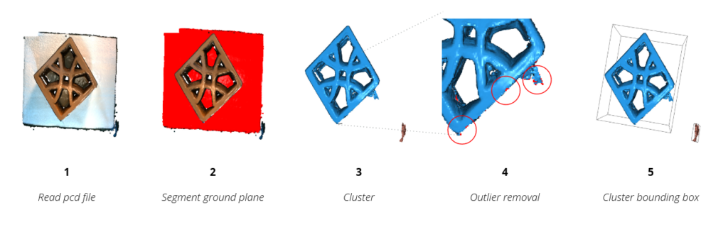
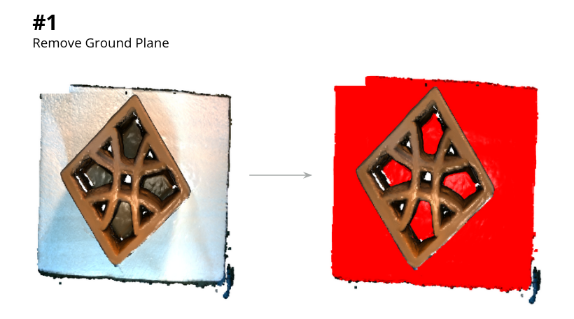
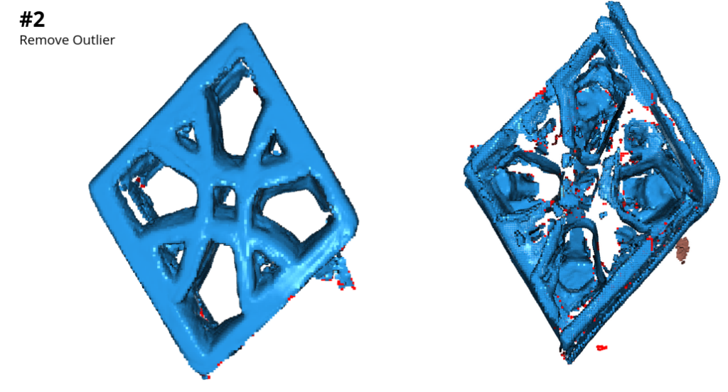
For the purpose of the project we chose these two steps from the ones mentioned above. This would lead us to get the most accurate scan point cloud in order to compare it with the 3d digital model. First we removed the base from the scan, and then we removed the outliers to get a more precise scan.
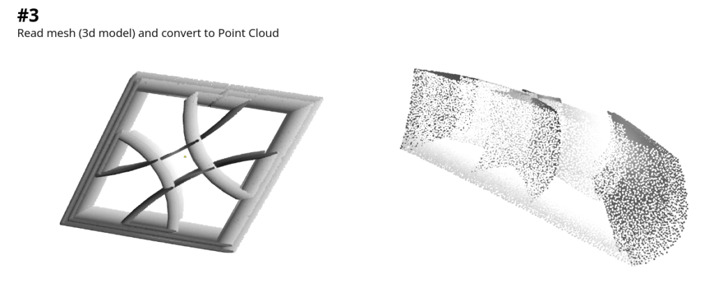
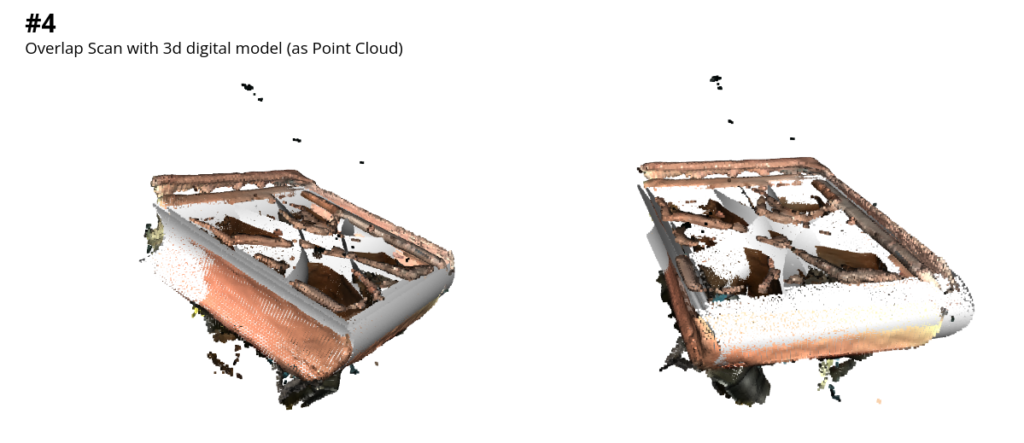
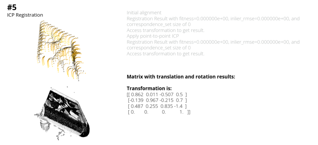
After these two first steps, we read the digital model in a point cloud to later on compare it with the scan point cloud (step number 4 shown below). With this data, we could finally get to the ICP Registration which was using several ros commands for the result. At the end, the transformation matrix result is shown. (How much did the piece change according to the scan and the 3d digital model point cloud comparison).