
Abstract
In this project, we explore how graph-based thinking can reshape construction planning by bridging design data and scheduling logic. Drawing inspiration from modular architecture and network theory, we investigate new ways to visualize, analyze, and optimize the sequencing of building elements. By combining insights from BIM, parametric modeling, and graph analysis, the work aims to uncover hidden patterns and critical relationships within the construction process—offering a more integrated and data-driven perspective on how buildings come together.
What If Your Building Knew Its Own Schedule?
Traditional construction scheduling, especially with methods like the Critical Path Method (CPM), focuses on identifying the longest sequence of dependent tasks. That determines the shortest time in which a project can be completed.
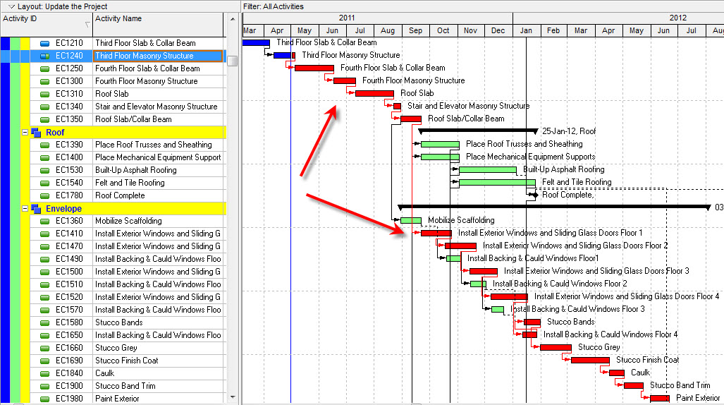
But buildings aren’t flat timelines—they’re spatial, layered, and modular. What if we mapped the actual building geometry to a network of tasks? What if every slab, column, or façade panel was a node in a graph, linked not just by duration but also by location and sequence?
That’s what we set out to do.
Our Strategy
We built a graph-based representation of a modular building system, where:
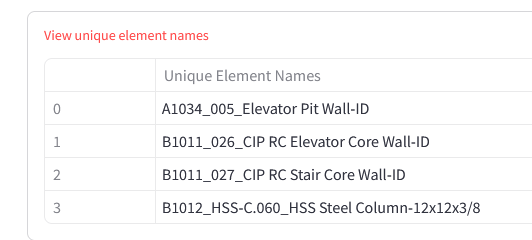
- Nodes represent individual IFC elements (e.g., slabs, columns, walls).
- Edges represent build dependencies, derived from structured WBS codes* and geometric relationships.
- Each node contains attributes:
- construction_sequence – a number defining build order,
- work_zone – spatial grouping by location,
- duration – estimated construction time from quantity take-offs and labor rates.
* Work Breakdown Structure (to be introduced in the next section)
Using this structure, we analyzed construction graphs in Neo4j to extract critical paths, uncover bottlenecks, and expose vulnerabilities in build logic. This wasn’t just a thought experiment – it was grounded in real geometry, material logic, and resource calculations. The value of this graph approach became especially clear in light of real-world challenges in industrialized construction – where sequencing and crane usage are major cost drivers. The observation that you can’t place 20 columns simultaneously with one crane isn’t just theoretical; it’s a daily constraint on site. Our graph structure begins to frame that problem quantitatively.
Methods and Tools
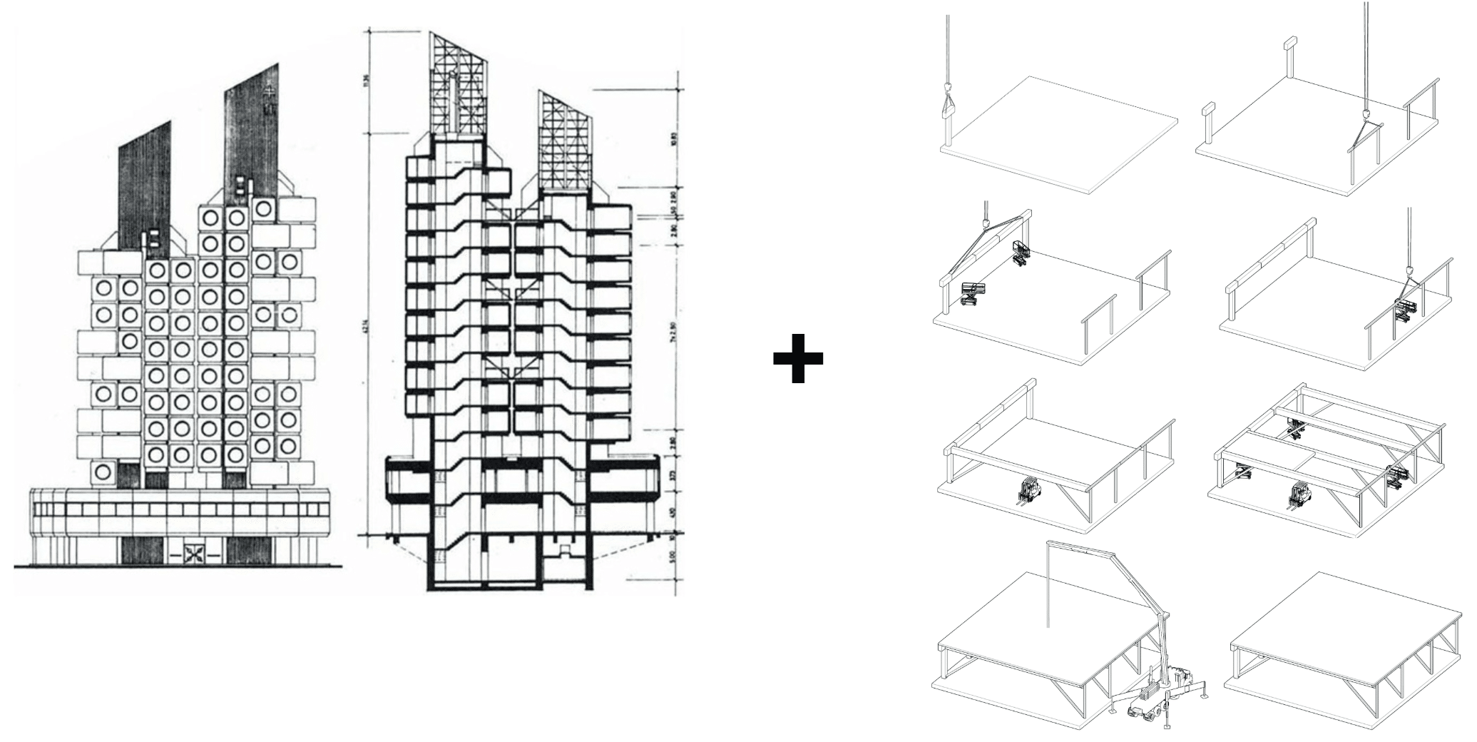
To implement this approach, we worked with a dynamic modular building case study, inspired by the Nakagin Capsule Tower and the Platform II system from Bryden Wood. The structure allows for easy assembly and disassembly and even delivering the full building in distinct, time-stretched segments, sub-volumes.
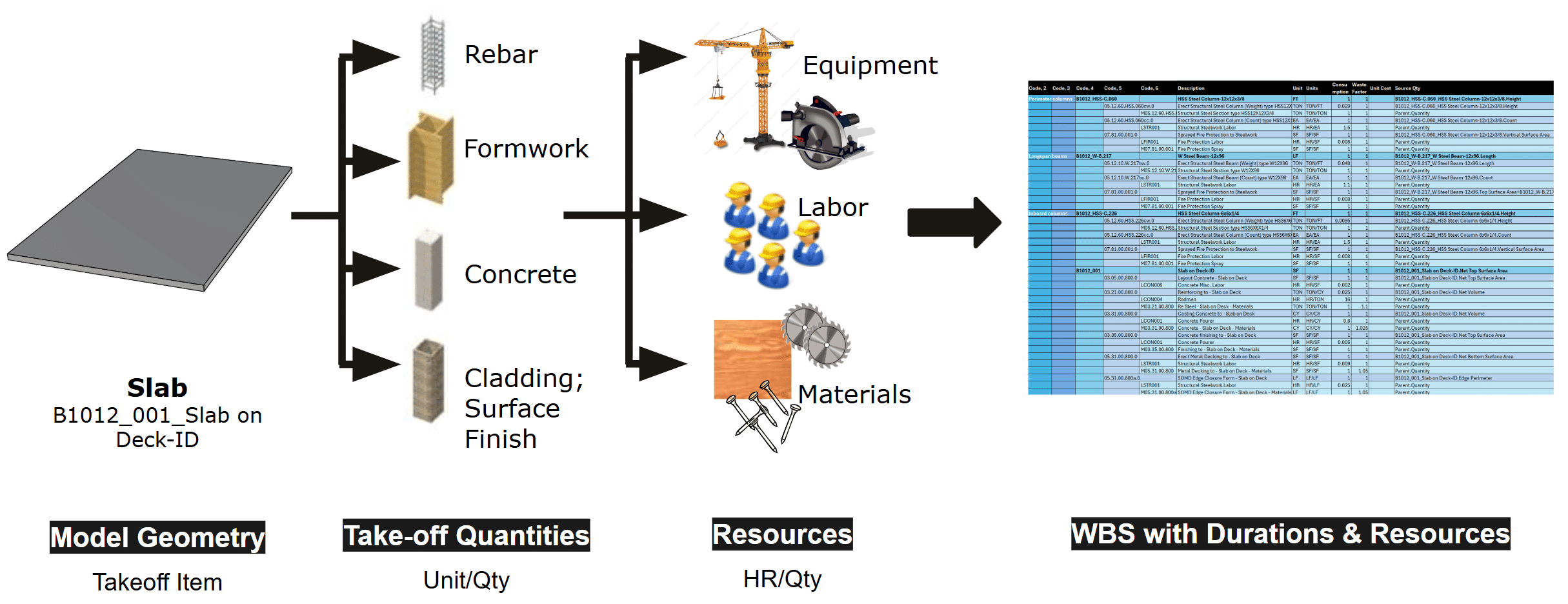
To populate those attributes our main aid is the Work Breakdown Structure (WBS), which is a hierarchical breakdown of all activities needed to build each element and the method to calculate durations and costs.
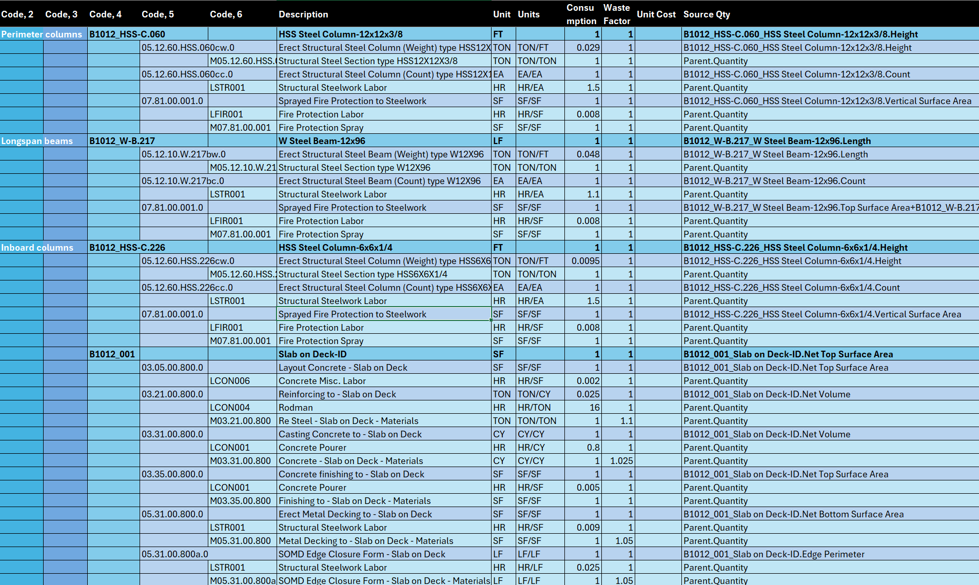
For each building element, it includes source quantities, labor and equipment needs, and hour/unit factors, making it the link between design, schedule, and resource planning.
At the onset of the AI Module we were shared with a robust Grasshopper definition, that aggregates modular building parts into a residential building block – Building Data Generator (BDG). In order to capture the complete construction schedule, we extended the BDG with a parametric building structure and envelope, as well as definitions to take-off the source quantities from the model.

Encoding Workflow: From IFC to Graph
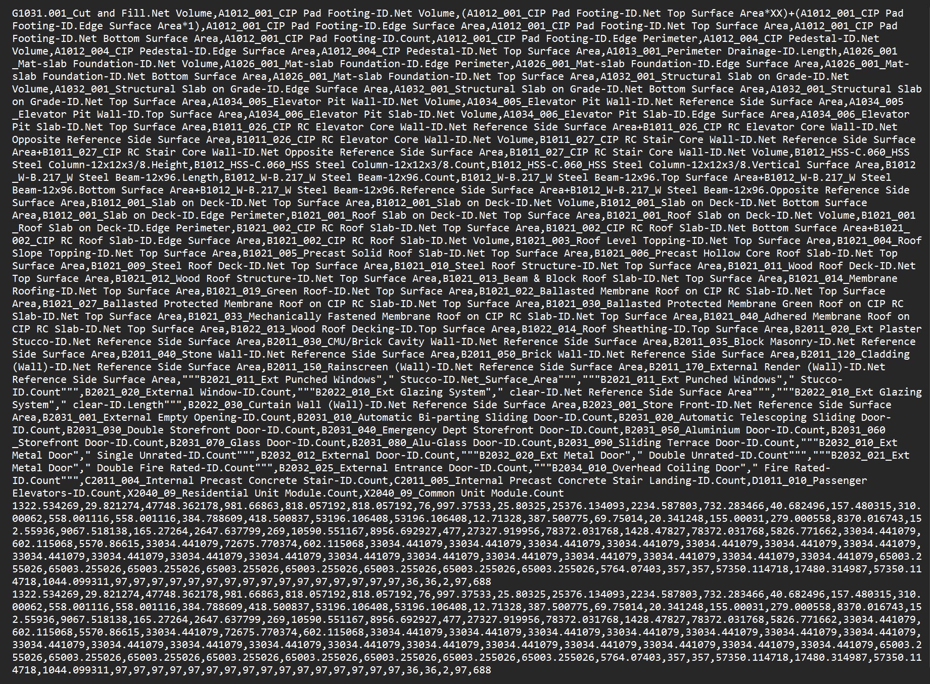
We had to encode non-quantitative scheduling logic as structured data for a graph that “makes sense” visually and analytically. Using the tools mentioned above, we went through a pragmatic process to transform the IFC into a graph-ready dataset:
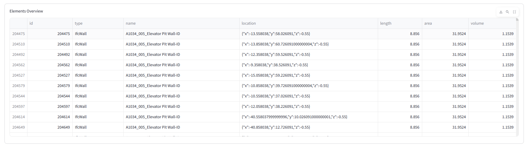
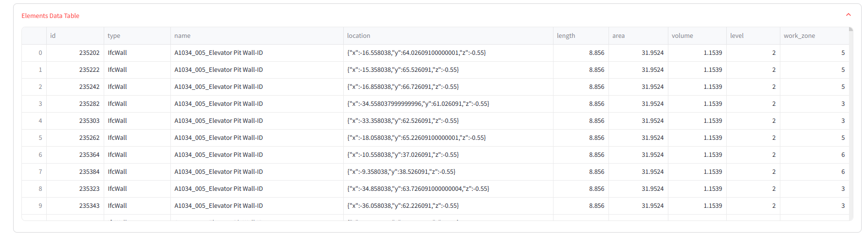
1. IFC Model Import
Our base model contained building elements tagged with WBS codes – these codes represent the activities related to the construction of the building element. These were mapped to construction_sequence integers to establish a build order.
2. Spatial Clustering
We used DBSCAN and KMeans clustering to organize elements:
DBSCAN grouped components by level.
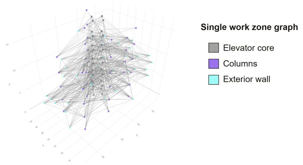
We used KMeans clustering on x and y coordinates to split IFC elements into six predefined work zones – defining vertical construction phases.
3. WBS Integration
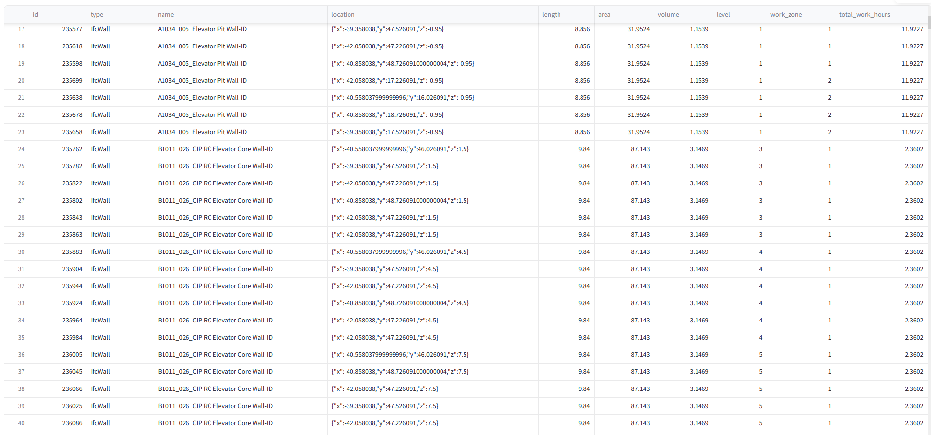
We merge WBS-derived data – sequence and duration – into each IFC element, combining it with work zone info. This extends the dataset, blending BIM geometry with construction schedule data into a single enriched model.
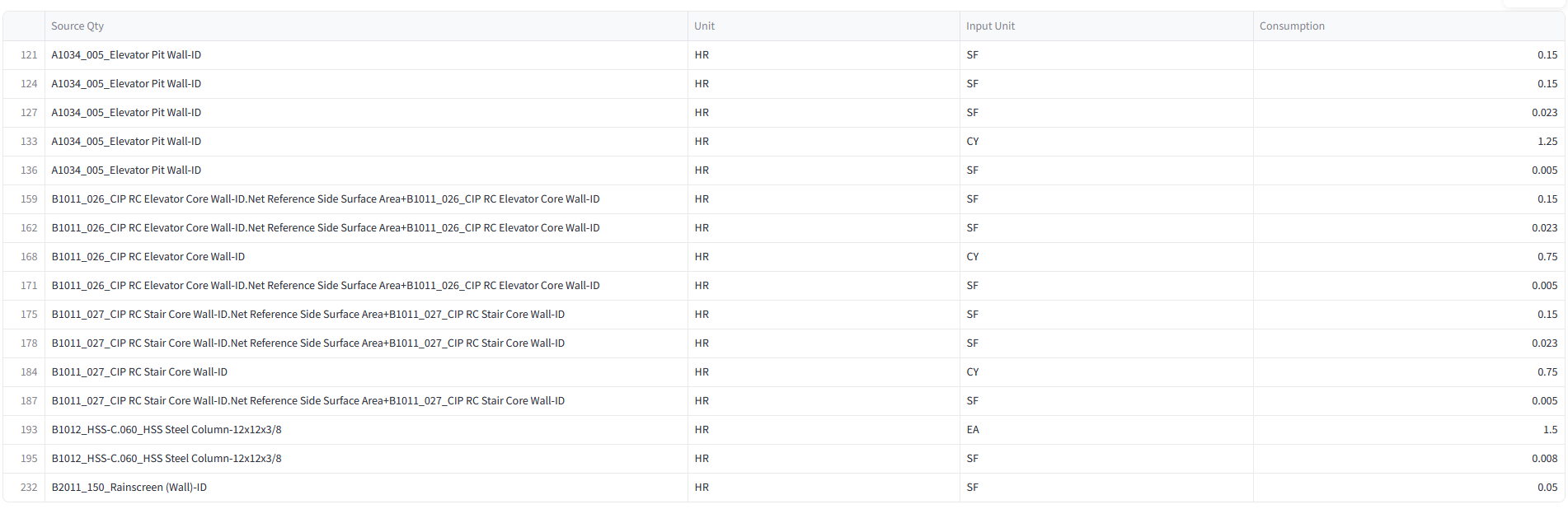
We filter the WBS to match our IFC model, focusing only on tasks linked to imported elements within a single work zone. This ensures a 1-to-1 match between WBS and model, creating a clean, consistent dataset for focused graph analysis.
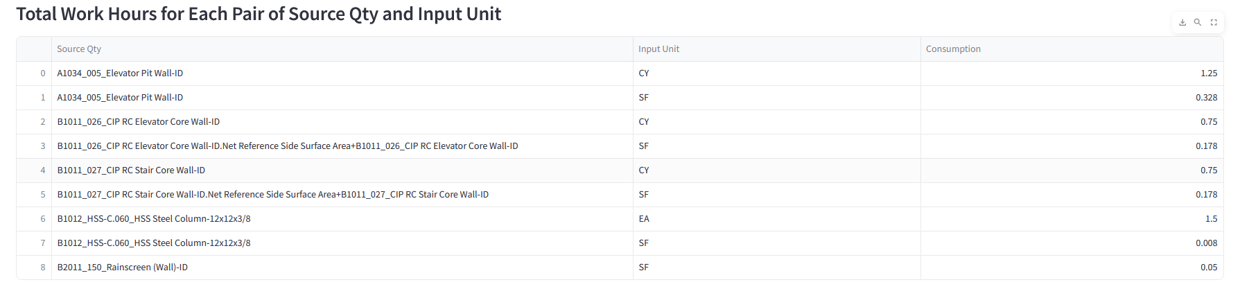
Before analysis, we calculate total work hours for each element using WBS resource rates and quantities. This sets accurate durations, sums crew demands per zone, and ensures the graph’s time weights are reliable for evaluating construction efficiency.
At this stage, every model element has a sequence number, duration, and work zone. We’ve built a dataset that links IFC with schedule data, ready for Neo4j graph analysis.
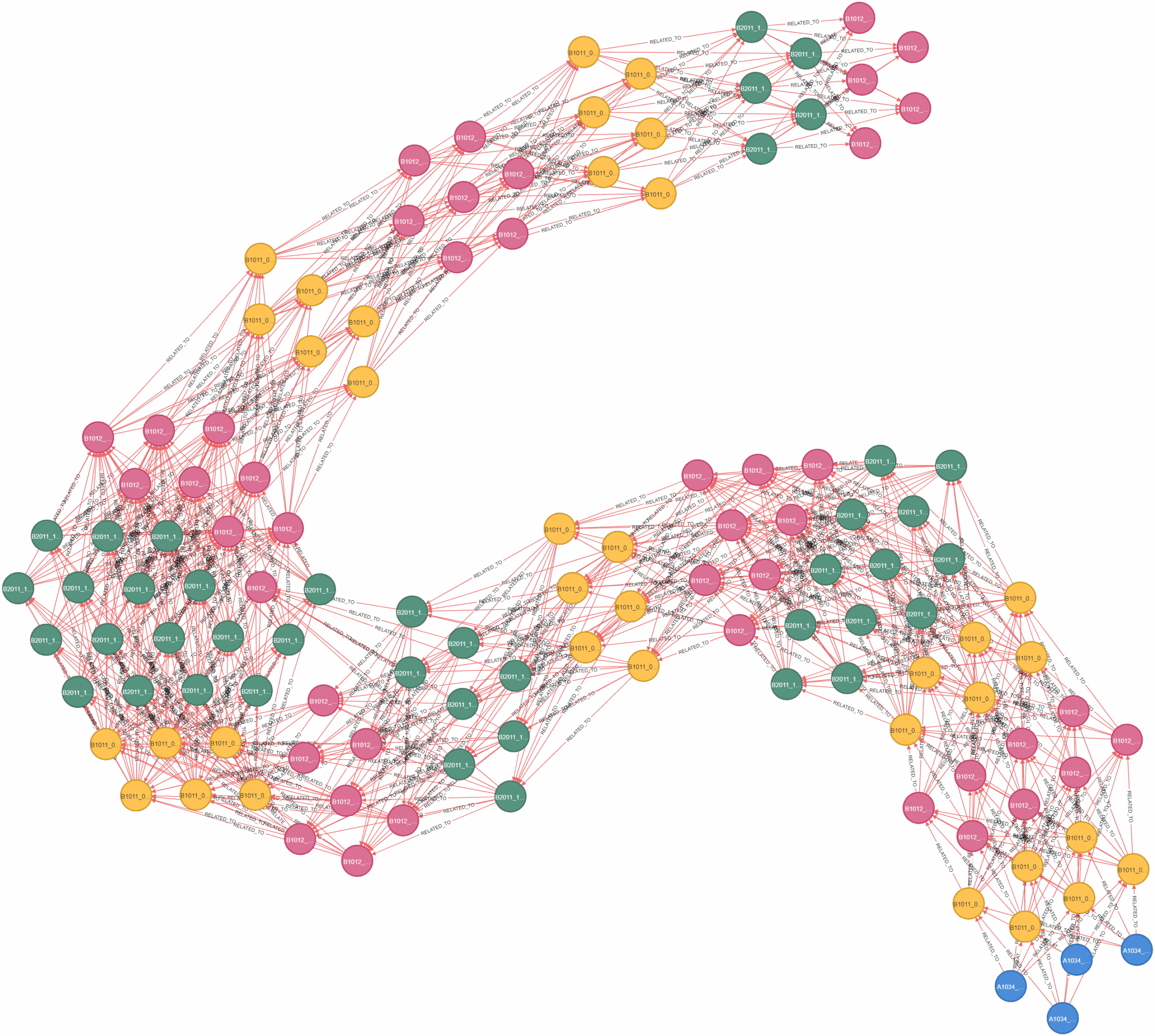
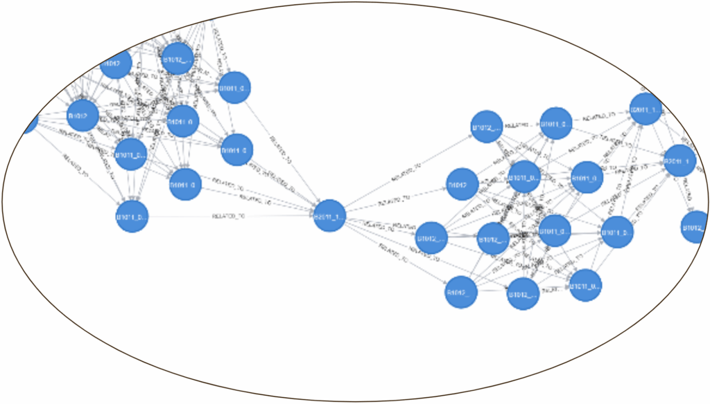
4. Graph Construction
The graph is directed and each edge represents a construction sequence dependency of the tasks required to be complete before the next task can be started. This created ribbons of concurrent tasks, which are color coded by their WBS sequence. You can clearly see patterns emerge, with groups before other groups.
Insights from the Graphs
In this enlarged callout, you can see the elevator pit walls in blue, causing dependency to the yellow tasks, elevator core wall construction.
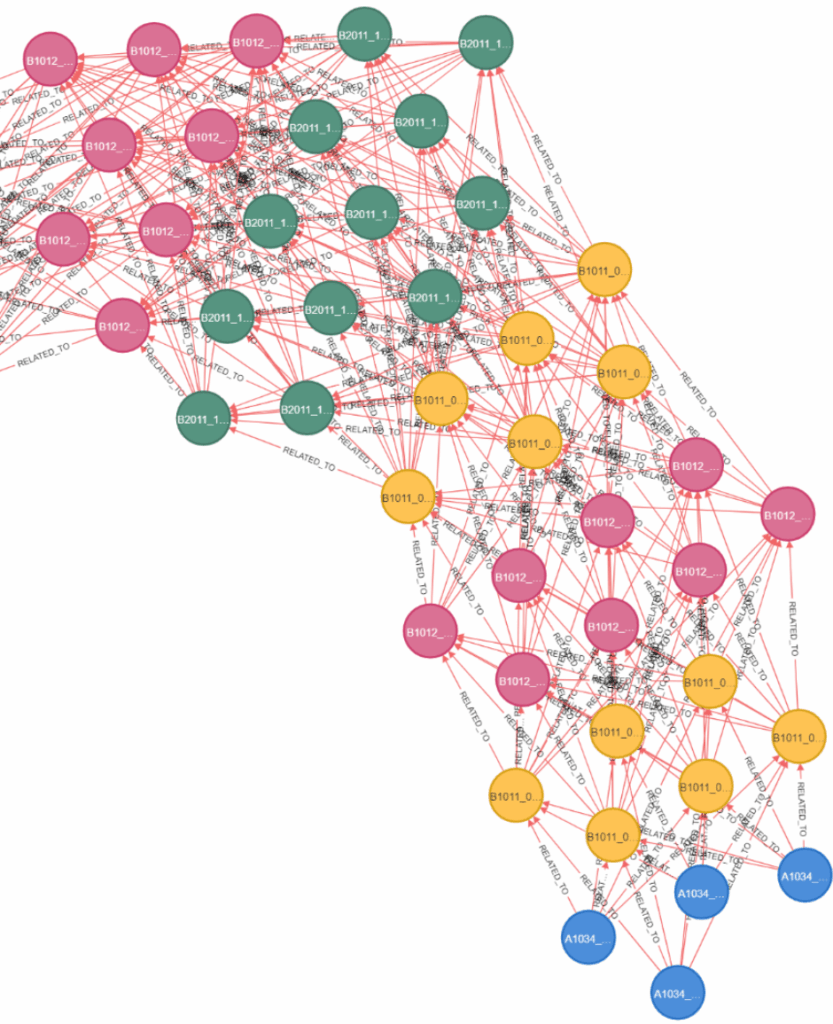
In this example graph output, we can see an unintended, but useful, result of our graph system, bottleneck tasks because visually apparent. If this task is not completed on time, the entire rest of the construction sequence is halted.
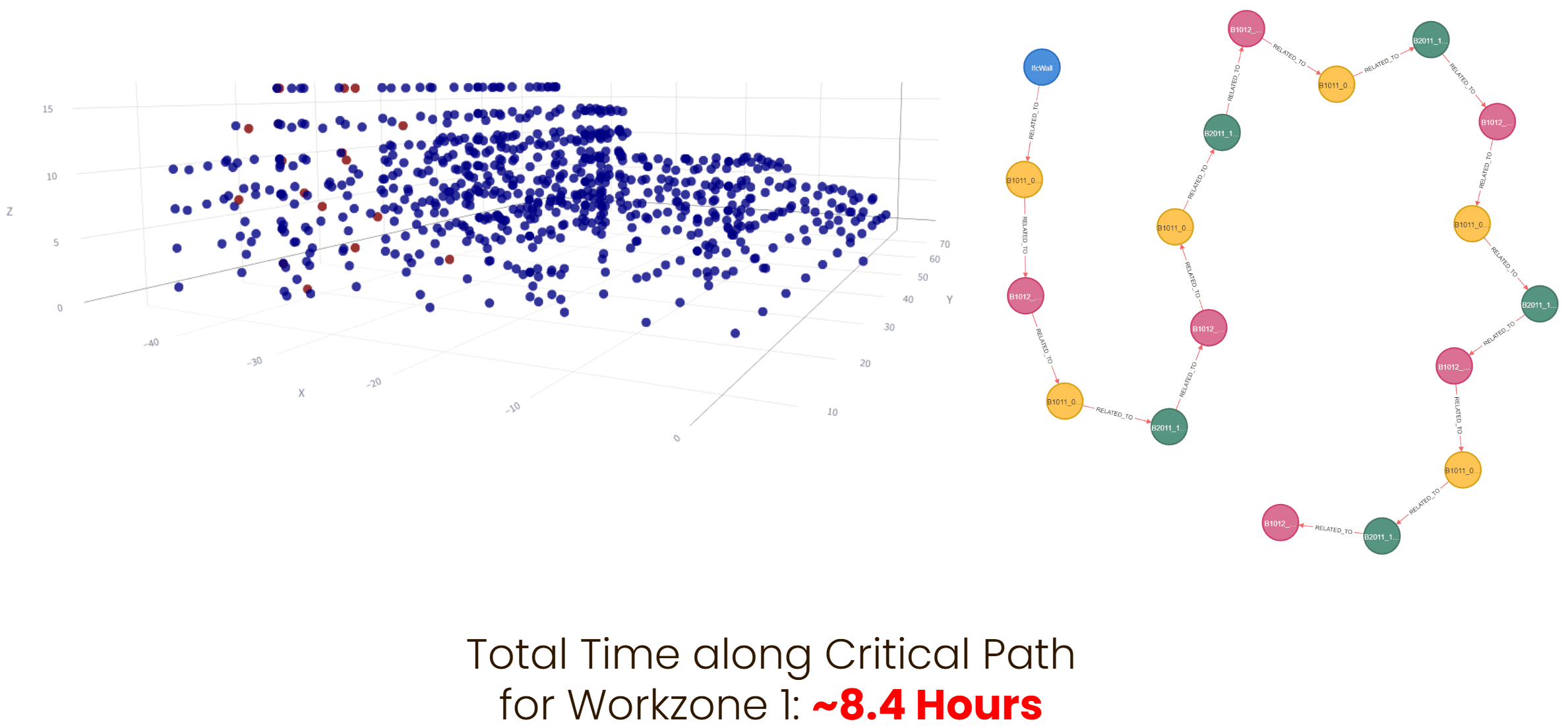
Neo4j Analysis
To find the critical path within our work zone we use the inverse time of construction to build our dependency edges. By inverting the time, we can use the Dijkstra shortest path algorithm instead as a longest path algorithm. We run this algorithm between the starting and ending nodes and add up the construction time incurred along each edge. In this work zone the critical path is expected to take just under 8 and half hours.
Conclusion and Takeaways
Our analysis does show the critical path through the graph and calculates a total time for all tasks on the path, however it also reveals flaws in our graph construction that clouds the flowline analysis. We can determine which tasks in each batch of tasks per level per work zone take the most time, however the process in which we build our graph assumes that all independent tasks can be performed concurrently. This imbues an unrealistic assumption that, for example, if there are twenty columns on the second level of the building, there are twenty cranes that can simultaneously place each of them. Future analysis could involve limits in building task batches into the graph construction or employ a traveling salesman style algorithm to move a limited amount of workers through the graph to limit. For example, if one limits the number of concurrent tasks when building the task chain, the result is much richer.
This project showed that graphs offer a powerful new lens for construction scheduling. Instead of treating time and space separately, we merged them into a unified, intelligent framework – linking IFC elements, construction logic, and resource planning into a single network. By grounding our graphs in real quantities and WBS data, we moved beyond diagrams into something actionable – something that could actually inform site management. If buildings could think, they’d speak in graphs, and now, maybe they do.
