Andromeda is a Rhino-native copilot that turns briefs, context, and massing into a single, interpretable graph so designers can enrich masterplans, evaluate KPIs, and bake results back to Rhino, without leaving their workflow.

Built for early-stage masterplanning, it aims to raise social value, connectivity, accessibility, and overall urban quality by unifying data, guiding program allocation, and providing instant, explainable feedback.

Why this matters

Masterplans lock in social & spatial choices for decades. Early stages are often rushed, data is fragmented, and feedback loops are thin, often yielding generic, non-contextual proposals.

Copilot, not autopilot. Andromeda keeps authorship with designers while adding speed and clarity. It reframes AI from generative “form spitting” to assistive decision-making via natural-language queries and interpretable graphs that flow back to editable 3D.

Graphs make values legible. By encoding streets, levels, plots, and programs as a network, the system exposes relationships, walkability, accessibility, diversity, compactness, GFA, and returns explainable KPIs you can compare across iterations and against the surrounding city.

Context counts. The proposed masterplan is merged with its direct neighborhood graph, so impact is measured where it matters: in the city. Thus the score is linked to the existing and not in isolation.

Aware of limits. KPIs guide iteration but don’t capture the full richness of urban life; data quality and graph-to-3D translation can introduce noise or biais, so human judgment remains central.

Pseudocode

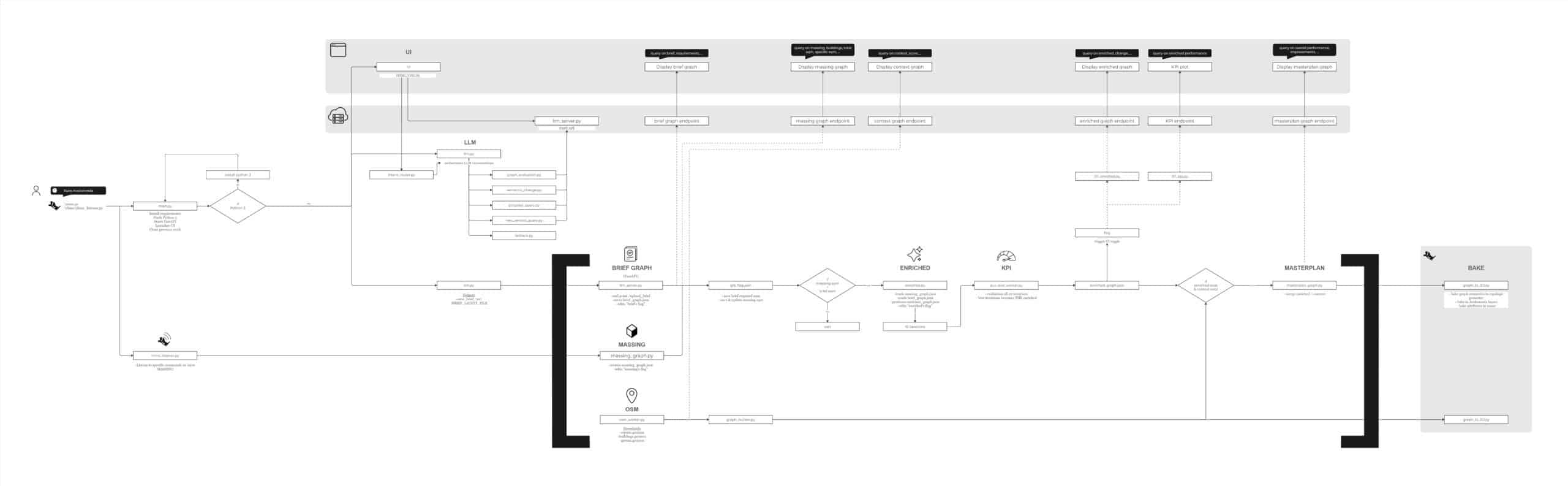
Andromeda runs through a single Rhino macro, which boots the whole system with two things: launches main.py and rhino_listener.py.
main.py then start multiple programs, first, a local FastAPI backend (llm_server.py) and opens the minimal web UI (index.html and related CSS and JS). The listener watches the specific ‘MASSING’ layer, debounces noisy edits, reacts to finished OSM jobs for context, and keeps tiny JSON flags in sync for preview and bake toggles.
We splitted the macro with 2 components as main.py retrieves Python 3, whereas rhino_listener.py rely on IronPython for baking geometries on the viewport.

Everything revolves around one slim graph shared between the backend, UI, and LLM. A few endpoints (/graph/, /preview, /bake, /llm/, /osm/*) handle I/O and triggers for the UI. The interface polls those endpoints, while the LLM answers through them, and Rhino stays the editing software.

High level architecture is as follow:

• input Context (OSM), Brief (PDF or text), and Massing (live from Rhino viewport) each are translated into graphs with respective technics.
• enrich Semantic data (program) is allocated from the brief onto the user’s massing topology, producing an interpretable, editable enriched graph.
• merge The proposal enriched masterplan is attached to its neighborhood graph, so impact is measured in the city, not in isolation.
• evaluation KPIs & explanations stream to the UI through the endpoints. Designers iterate or Bake iteration / results back to Rhino with tags and attributes intact.
• chat Natural-language queries route to data-backed actions, never overwriting geometry without the user’s input.

How it works

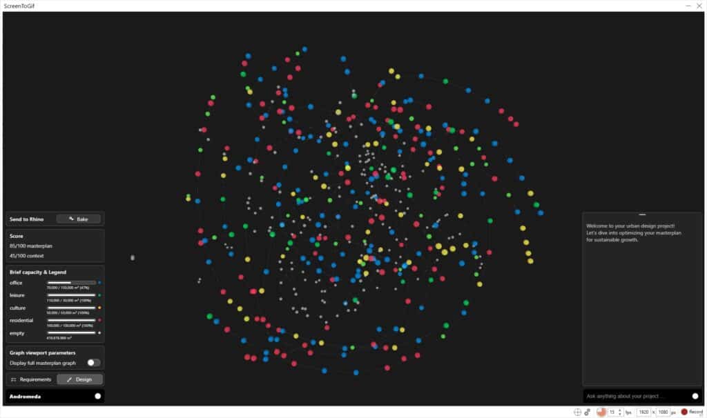
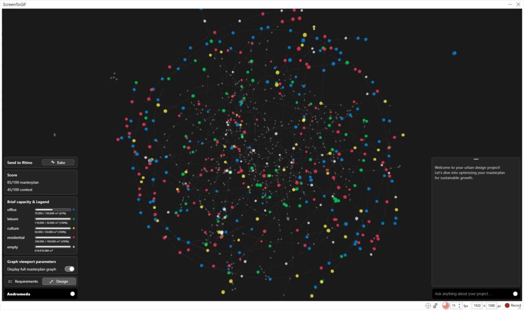
UI

Behind the appearance of this UI many things are going on: HTML/CSS/JS to create it, we use a FAST API local server where we connect our graphs, RT calculations, the LLM and visualization of the graphs using a three.js & webGL graph viewer.

Context Graph

The context is imported from OpenStreetMaps trough OSMnx asking the coordinates and a radius to the user. Then the data will be simplified and distributed into program nodes, buildings and streets to build the context graph. In paralel the downloaded geometries will be baked in the Rhino viewport for contextual reference.

Brief to semantic graph

The user can upload the brief as PDF either with the button or through the chat. Then, it is uploaded via /upload_brief. The server, running through llm_server.py, retrieves the text and directly calls the function extract_graph_from_brief(), which prompts the local model (LM Studio in our case) to return a program graph formatted in JSON following with: nodes: {id, label, typology, footprint, scale, social_weight} combined with metadata and edges: {source, target, type {[“contains”,”mobility”,”adjacent”], mode: []}.
The result is stored next to the brief with date and time and mirrored as a copy in knowledge/briefs/brief_graph.json for easier access and exposed through an endpoint for later enrichment and also for chat context during queries.

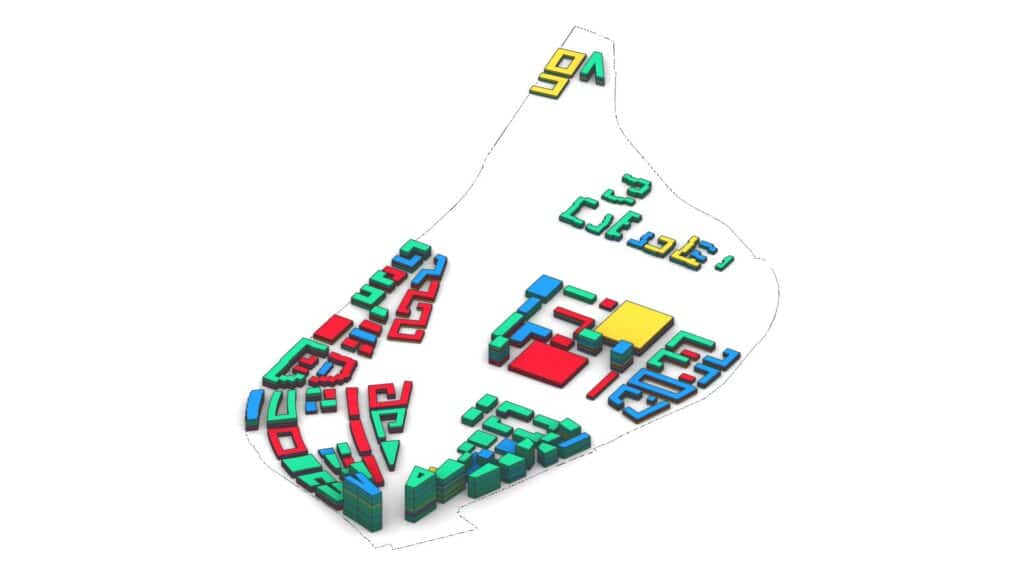
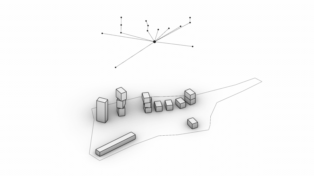
Massing to topological graph

This is enabled by the file massing_graph.py, through the MASSING layer and its sublayers, where the designer should draw. Geometries are converted to Breps, sectioned into height spans, and each span is intersected to produce level contours. Each level area is computed and it’s data is saved in the corresponding node, while edges connect consecutive levels creating the building.

Buildings are grouped either by touching bounding boxes or by sublayer, avoiding accidental merges of separate masses.

Then, a branching is introduced when a mass splits (e.g. a podium with multiple towers), branches are identified from XY section connectivity and given stable branch_ids. Additional edges connect the podium and tower nodes.

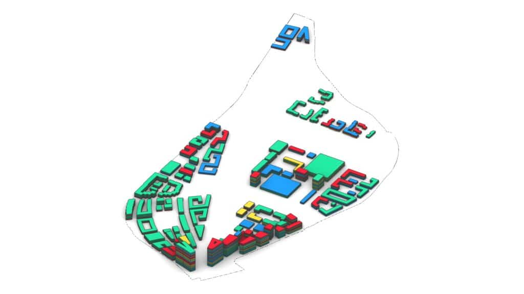
Program Enrichment

Only when the brief’s requirements in sqm are fulfilled by the massing the system allows to compute the enrich script. 

After that to insert program, enrich divides both the brief and massing in smaller parts. A stochastic assignment dispatches the program with predefined preferences inside the topological graph and calculates the main program of the node for evaluation.

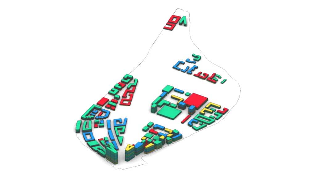
Merging Masterplan with context

The merging process is implemented through the script masterplan_graph.py which operates as the link between the enriched massing graph and the imported context data. The process to make it is as it follows:
masterplan_graph.py merges an empty-plot context graph (outside boundary) with the enriched massing graph. Instead of a synthetic hub, it detects connector street nodes at the site edge and attaches them to the nearest massing node (prefer street nodes, fall back to levels) with type:”access” edges, within a configurable distance (default 50 m). The final masterplan graph is written to knowledge/merge/masterplan_graph.json with basic collision-safe node ID renaming.

KPI Evaluation

All these conclusions are taken into account inside our repository as follow: evaluation/aux_eval_worker.py implements the computation of urban KPIs directly on the enriched graph. It assigns each typed node (residential, office, cultural, leisure and green) a weight and pairs it with compatible values. Distances are measured between typed nodes inside connected components or to their nearest street anchors, using Dijkstra shortest paths with a cutoff radius of 3000 m. For every valid pair, a score contribution is accumulated as (Ki * Kj * Fij) / dij. The average per pair is scaled *1000 and normalized against empirical bands, producing a verdict (low, acceptable, good,
great). Results are exported as JSON in each folder under knowledge/osm/ , and testkpi.py validates the stability of these values against reference city benchmarks.

LLM

Every query that the designer sends to the copilot is processed through LM Studio, which runs two complementary models. For the embedding stage we use Nomic Embed Text v1.5, a model chosen for its stability and efficiency in representing the meaning of short prompts. Once the routing is decided, the query may trigger internal computations or, when a natural language answer is required, it is passed to the main LLM. We’ve incorporated 5 query types: brief queries, graph queries, semantic change queries, new versiono queries and fallback queries (for more general answers inside our context).

Graph to 3D

This process compares the cache layers to the enriched graph’s attributes. Then, we bake the enriched geometry with new semantic attributes, namings, colors and layer according to the program.

From MCP, v0, v1

This thesis has seen strong development and progress with a few versions. Here, we will develop the process and techniques used from the Minimum Coherent Prototype (MCP) to the piece of software: Andromeda.

Case studies

Jernbanebyen, Copenhagen by COBE

Cortex Park, Odense by Nord.

Potential

Andromeda’s real promise is to speed up early masterplanning iterations without surrendering authorship, and to put social value back in the loop. With natural-language queries on a graph, designers get quick, data-backed suggestions while staying in full control of the model. Because proposals are merged with their surrounding neighborhood, decisions become city-aware: walkability, accessibility, diversity, compactness, and GFA compliance are measured where they actually matter, not in isolation.



The feedback is explainable and grounded in truth. The same graph you’re shaping produces the KPIs, quietly, as you work. Trade-offs stay in plain sight across iterations, and results bake straight back into Rhino as tagged, enriched, editable geometry.



With a clear path to a packaged plug-in and stronger stability, the prototype can mature into a maintainable tool for practice, helping teams embed social and ecological values in everyday design workflows rather than as afterthoughts. More broadly, Andromeda shows that graphs are a powerful way to add value to existing workflows.

What’s next

The current state of Andromeda is sconsidered as V1 or “Alpha build”. Many steps have to be considered before shipping a flexible product. We highlighted a few next steps we would develop:

• Brief to graph more robust. We could fine-tune the LLM for briefs and widen action coverage via embeddings so parsing is faster and more reliable.
• Geometry-aware enrichment. Support variable floor heights and podiums (taller ground floors), so allocations reflect more various and real structural / programmatic variation.
• Richer KPIs. Extending the scores beyond the social and going toward sustainability, placemaking, and visual quality could be possible development. Also, if ML gains were not relevant on simple score computing, a more comlpex KPI could benefit from ML once a solid dataset created.
• Stronger data contracts. Harden the pipeline against noisy OSM/brief inputs and JSON hiccups.
• Graph to 3D fidelity. Improve round-trip baking and attribute mapping so enriched graphs come back to Rhino with fewer distortions and even clearer tags.
• City-scale benchmarks. Keep normalizing scores against multiple cities to situate the masterplan proposals within real urban patterns.

References

1. Araya, D. (2023). Smart cities and AI: Copilot or autopilot? Springer. https://doi.org/10.1007/978-3-031-35472-8
2. Batty, M. (2013). The new science of cities. MIT Press.
3. Boeing, G. (2017). OSMnx: New methods for acquiring, constructing, analyzing, and visualizing complex street networks. Computers, Environment and Urban Systems, 65, 126–139. https://doi.org/10.1016/j.compenvurbsys.2017.05.004
4. Du, J., Zheng, Y., Liu, Y., & Liu, H. (2022). Machine learning for urban planning: A review. Cities, 131, 103889. https://doi.org/10.1016/j.cities.2022.103889
5. Gehl, J. (2010). Cities for people. Island Press.
6. Giuffrida, N., et al. (2024). On the equity of the x-minute city from the perspective of walkability. Transportation Engineering, 16, 100244. https://doi.org/10.1016/j.treng.2024.100244
7. Gu, X., et al. (2023). Generating urban road networks with conditional diffusion models. ISPRS International Journal of GeoInformation, 13(6), 203. https://doi.org/10.3390/ijgi13060203
8. Hillier, B., & Hanson, J. (1984). The social logic of space. Cambridge University Press.
9. Jiang, F., & Ma, J. (2025). Environmental justice in the 15-minute city. Smart Cities, 8(2), 53. https://doi.org/10.3390/smartcities8020053
10. Karimi, K. (2018). Space syntax: Consolidation and transformation of an urban research program. Journal of Space Syntax, 9(1), 17–38.
11. Leach, N. (2021). AI and design authorship. Architectural Design, 91(4), 6–13. https://doi.org/10.1002/ad.2684
12. Leach, N., & Scott, P. (2022). Architecture in the age of artificial intelligence. Bloomsbury.
13. Marshall, S. (2012). Planning, design and the complexity of cities. Routledge.
14. Nagy, D., Lau, D., Locke, J., Stoddart, J., Villaggi, L., Wang, R., Zhao, D., & Benjamin, D. (2017). Project Discover: An application of generative design for architectural space planning. In Proceedings of the 37th Annual Conference of the Association for Computer Aided Design in Architecture (ACADIA) (pp. 106–113). ACADIA.
15. Negroponte, N. (1970). The architecture machine. MIT Press.
16. Porta, S., Crucitti, P., & Latora, V. (2006). The network analysis of urban streets: A dual approach. Physica A: Statistical Mechanics and its Applications, 369(2), 853–866. https://doi.org/10.1016/j.physa.2005.12.063
17. Terzidis, K. (2006). Algorithmic architecture. Routledge.
18. Vasturiano. (n.d.). 3D Force-Graph. GitHub. https://github.com/vasturiano/3dforce-graph