ML-Driven Plant Placement for Adaptive Architecture
BioSpatial Intelligence explores how machine learning can support planting decisions in architectural spaces. The project starts from a simple design question: when we design a building, how can we decide which plants belong to which environmental conditions? Instead of relying only on intuition, we developed a workflow that reads the microclimate of a building and predicts the most suitable plant cluster for every tile of the floor plan.
From Building Geometry to Environmental Data
Sun · Radiation · UDI
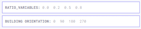
The first step was to create a parametric dataset in Grasshopper. Different building configurations are created by changing the building orientation and window ratios on each façade. Each scenario was subdivided into a 10×10 tile grid, creating 100 spatial units per configuration.
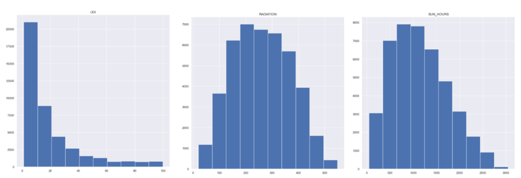
For every tile, we simulated environmental values such as sun hours, radiation, useful daylight illuminance and humidity proxy. This allowed us to describe each part of the floor not as a generic space, but as a specific microclimate with its own environmental behavior. (Python & Honeybee)
Engineering Spatial Features
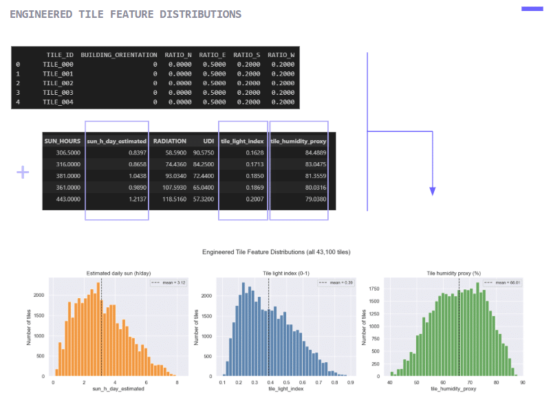
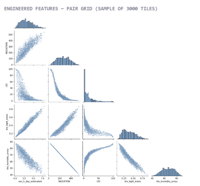
Raw simulation outputs were then transformed into comparable features. Annual sun hours were converted into an estimated daily sun value, while radiation, sun and daylight were combined into a tile light index. A humidity proxy was also derived to compare spatial conditions with plant requirements.
This step was important because plants and architecture speak different languages: simulations describe spaces, while botanical data describes environmental needs. Feature engineering helped create a shared language between the two.
Understanding Plant Needs Through Clustering
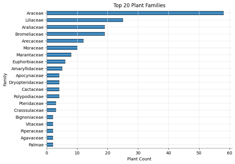
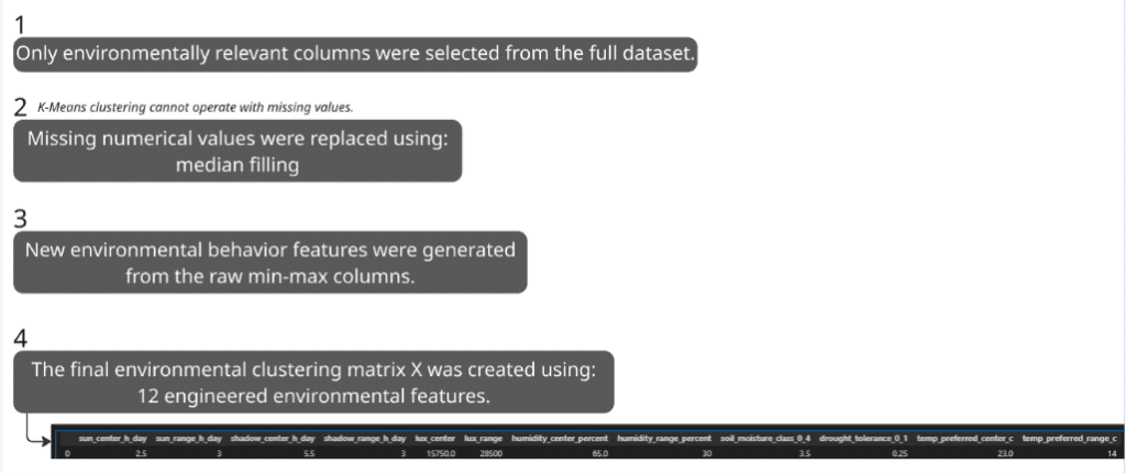
On the plant side, we cleaned and prepared a dataset of plant requirements (which was taken from Kaggle). Instead of assigning plants manually, we used environmental features such as sunlight, shadow preference, lux range, humidity, soil moisture, drought tolerance and temperature tolerance.
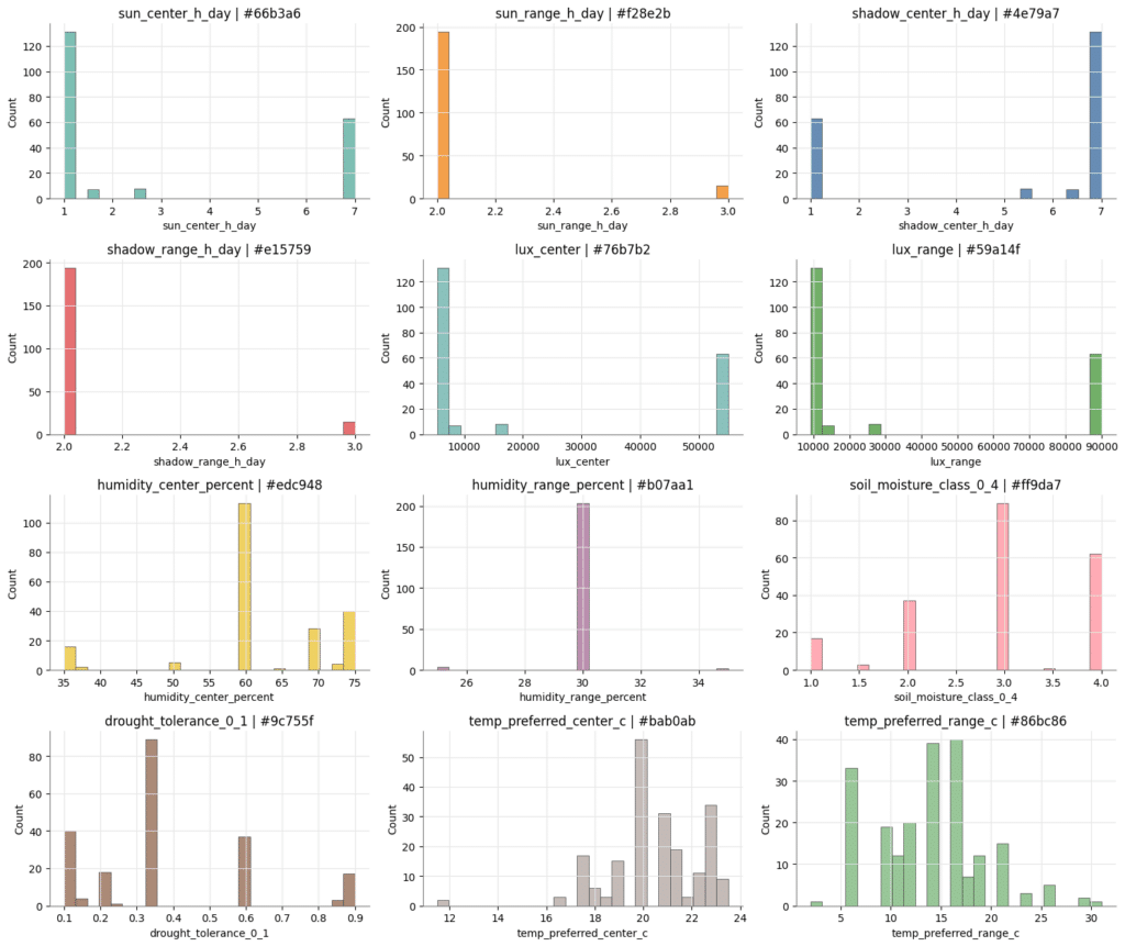
The data should be scaled because the features have very different value ranges.
After scaling the data, we tested different numbers of clusters using elbow and silhouette scores. The final result was a set of seven plant clusters, each representing a different environmental profile. These clusters were then interpreted through familiar plant examples, such as Golden Pothos, Snake Plant, Jade Plant, Peace Lily, Boston Fern and others.
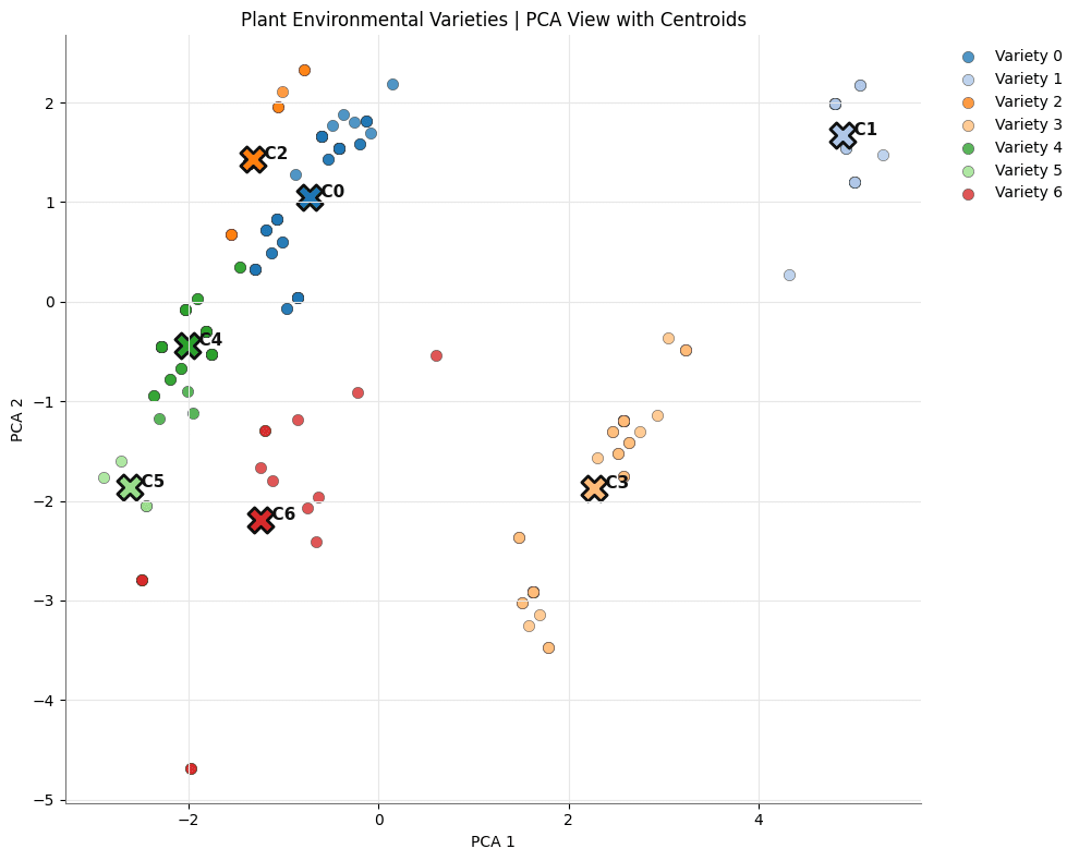
PCA, visualizing the clusters.
Matching Tiles with Plant Clusters
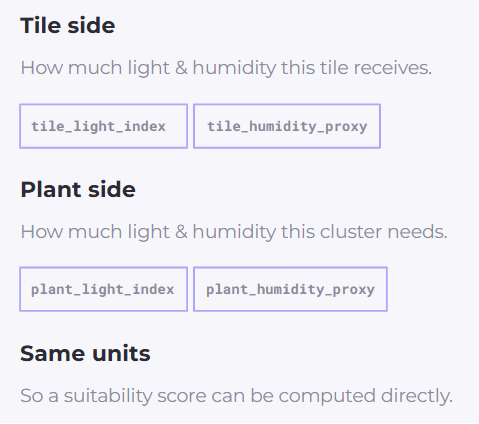
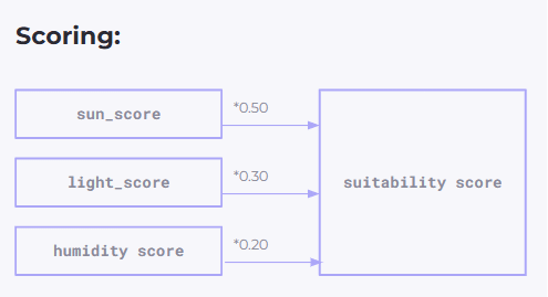
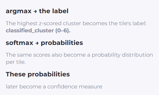
Once both sides were encoded, the next step was to match tiles with plant clusters. Each tile had environmental values, and each plant cluster had environmental preferences. A suitability score was calculated by comparing the tile conditions with the plant cluster requirements.
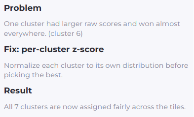
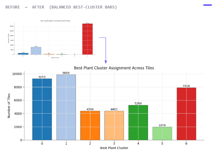
At first, one cluster dominated the results because its raw scores were naturally higher. To solve this, we normalized each cluster score using a z-score method. This allowed all seven clusters to compete more fairly and produced a more balanced spatial distribution across the floor plan.
Creating the Final Labeled Dataset
Training the Machine Learning Model
We then trained machine-learning models to predict the best-fit plant cluster directly from building and environmental features. The input features included building orientation, façade ratios, UDI, sun hours and radiation. The target label was the classified plant cluster.
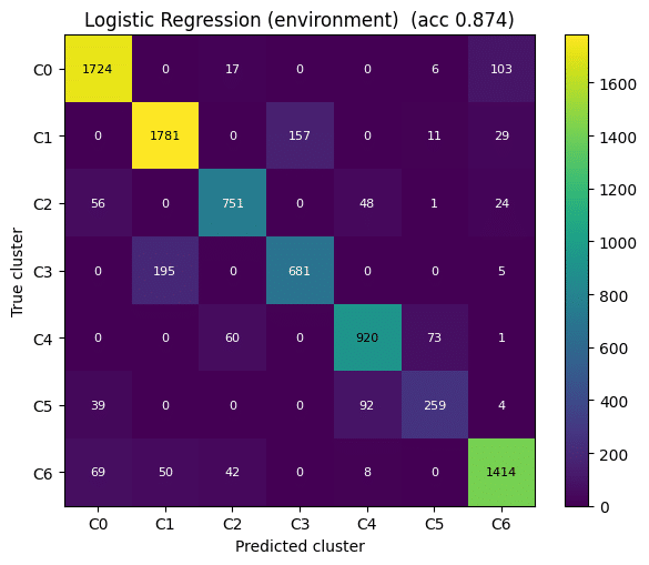
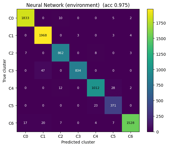
We compared Logistic Regression and a Neural Network model. While Logistic Regression provided a useful baseline, the Neural Network performed significantly better, reaching approximately 97.8% accuracy. This showed that the relationship between spatial parameters and plant suitability was learnable and could be used as a predictive design tool.
LOGISTIC REGRESSION
8 environmental & geometric inputs
Each tile’s raw conditions, used to predict its plant cluster
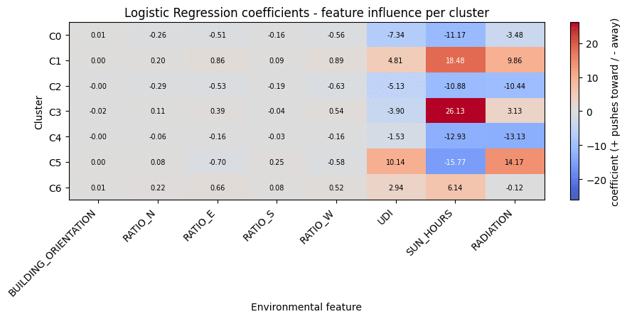
The coefficients show what drives it
Sun & radiation dominate.
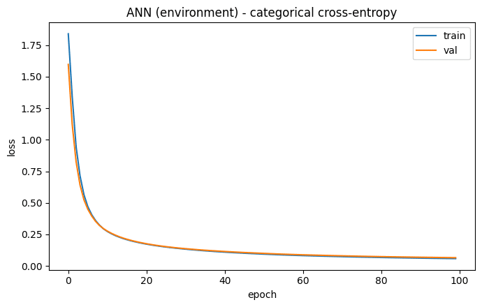
NEURAL NETWORK
Keras, 16 → 16 → 7
Two hidden layers, softmax output.
~97.8% accuracy
10-point jump over above Logistic Regression.
Deployment in Grasshopper
The trained model was then deployed back into Grasshopper. For a selected building configuration, the model predicts the suitable plant cluster for each of the 100 tiles and visualizes the result as a colored floor map in Rhino.
This step transforms the workflow from a notebook-based analysis into a live design tool. Designers can change architectural parameters and immediately see how the recommended planting strategy changes across the space.
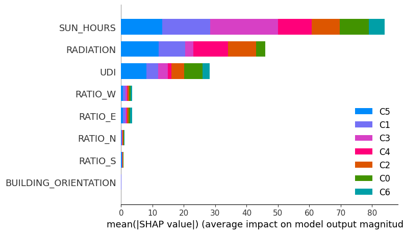
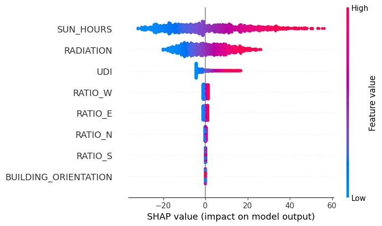
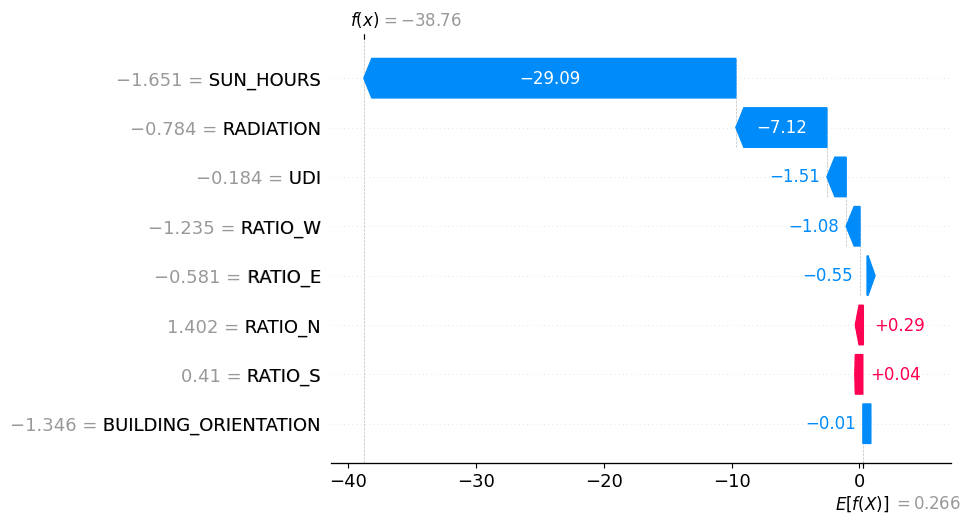
Explaining the Model with SHAP
To make the model more transparent, we used SHAP analysis. This allowed us to understand which features had the strongest influence on the predictions. The results showed that sun and radiation were the dominant drivers, followed by daylight, while façade ratios had less direct importance.
This was important because a machine-learning model is more useful for designers when its decisions can be explained. SHAP helped us move from prediction to interpretation, showing why a specific tile was assigned to a specific plant cluster.
Toward an Interactive Design Interface
The final phase of BioSpatial Intelligence is to turn this workflow into an interactive interface. Instead of working directly inside Grasshopper or code, the designer would be able to adjust building parameters through a simple interface and receive real-time plant recommendations.
In this sense, the project is not only a classification model. It is a prototype for an adaptive design assistant: a tool that connects environmental simulation, botanical intelligence and machine learning to support more responsive architectural interiors.