Objective
Traditional flood risk maps take months to produce, are updated only every few years, and are too coarse, they might say a whole district is at risk without telling you which specific street or field will actually be underwater.
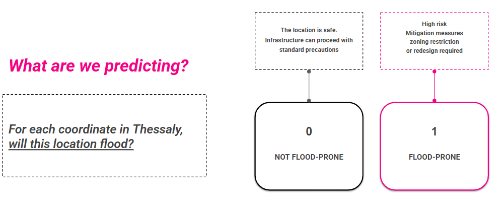
“We are going to predict whether any given location in Thessaly, Greece is Flood-Prone or Not Flood-Prone using binary classification and machine learning.”
Thessaly Background
Thessaly is one of Greece’s most flood-prone regions. The catastrophic 2023 Storm Daniel flood brought up to 750mm of rain in Zagora in just 24 hours the equivalent of months of rainfall in a single day
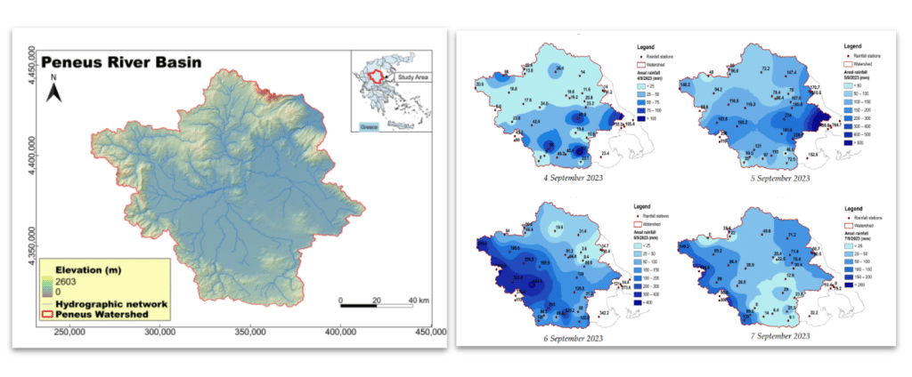
Left: Geomorphological map of the study area–Peneus river basin—along with its main hydrographic network. Coordinate System: GGRS87/Greek Grid (EPSG:2100).
https://www.itia.ntua.gr/el/getfile/2562/1/documents/water-17-02678-v2.pdf
Rigth: Spatial distribution of daily rainfall depths during the propagation of Storm Daniel.
https://www.itia.ntua.gr/en/getfile/2451/1/documents/water-16-00980.pdf
Data Preparation
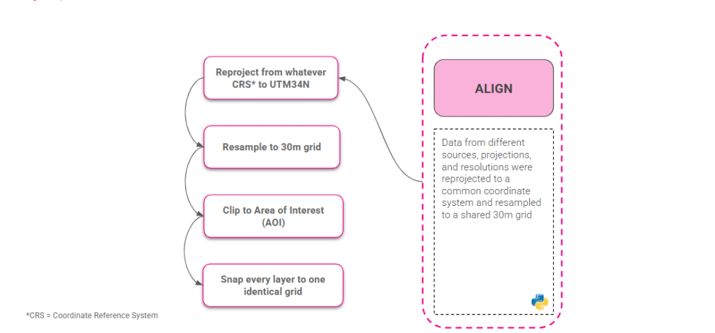
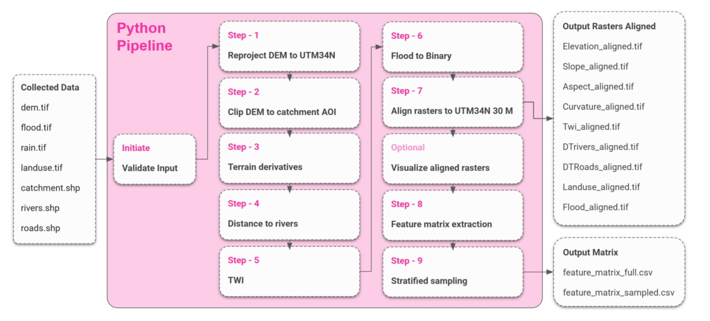
We pulled together elevation, river and road networks, land use, and rainfall and flood data, then aligned and sampled them for training. The Data preparation workflow was the most critical step of the workflow, making spatial alignment the essential foundation for all subsequent analysis. We reprojected every layer to a common coordinate system and resampled to a shared 30-metre grid, so the data lines up cell by cell. From roughly 12 million catchment cells, we drew our training sample.
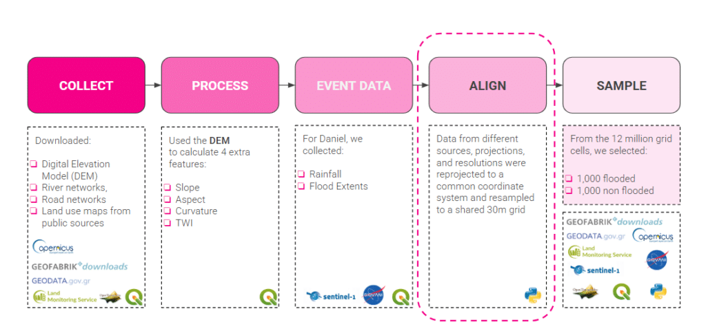
To enable testing across regions, we designed a nine-step reproducible Python pipeline handling reprojection, clipping, terrain derivation, distance and wetness metrics, flood binarisation, alignment, and sampling.
Data Pipeline
Features
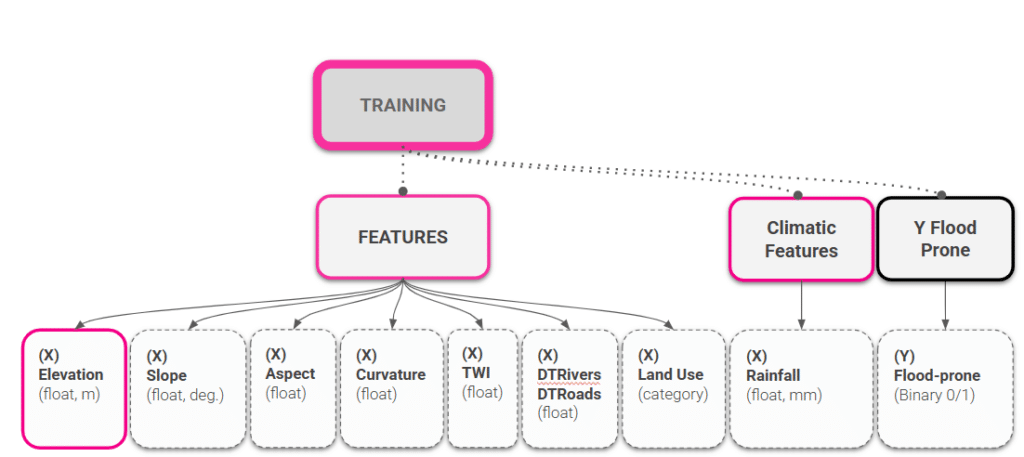
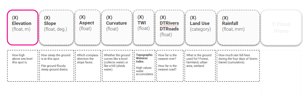
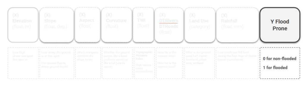
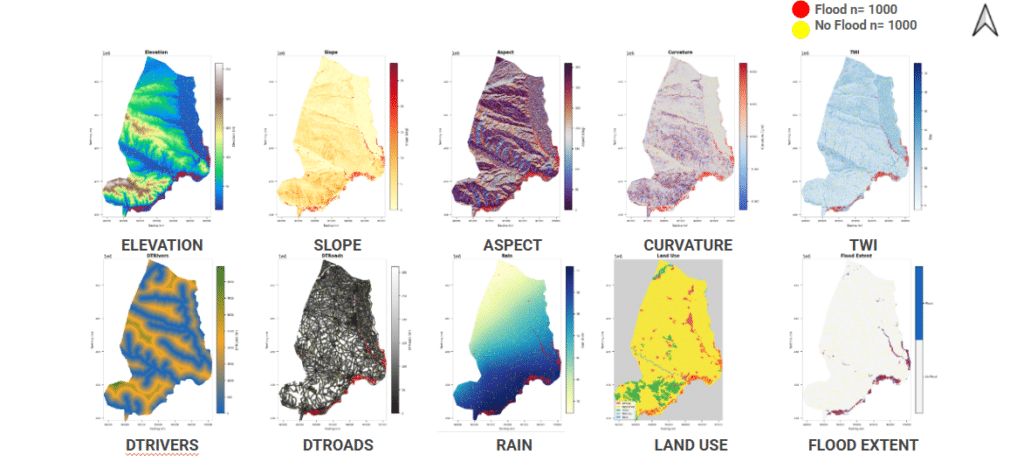
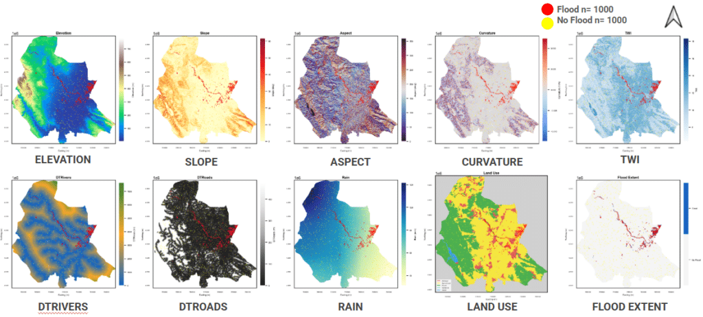
We shift to training preparation, selecting a total of 9 features to drive our flood prediction model. Five come from terrain — elevation, slope, aspect, curvature, and the Topographic Wetness Index (TWI), which captures where water collects. Two are distances — to the nearest river and the nearest road. Then land use, and the event rainfall.
Training & Testing Split
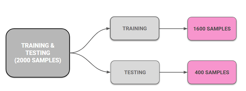
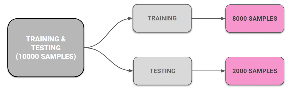
We built a data set of 2000 points, 1000 flooded and 1000 non flooded. We then split the data the usual way 80% to train on, 20% held back. So the model learns from 1,600 points and gets tested on 400 it’s never seen.
Pretraining Conclusions
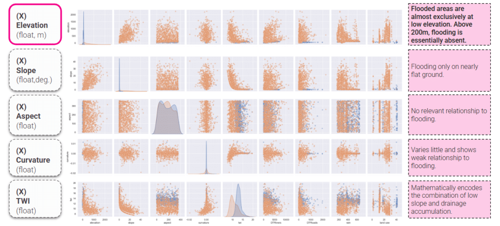
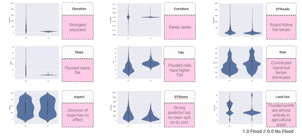
Then we just looked at the data first. These pairplots below are the terrain features and we can see that all the flooding happens below 200 meters, on flat ground. Which way a slope faces doesn’t matter, curvature barely moves, and TWI mostly just repeats what elevation and slope already tell us.
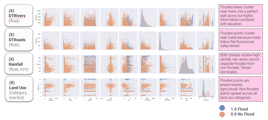
The flooded points sit close to rivers and roads, and they’re almost all on farmland. Rain on its own can’t tell flooded from dry.
The violin plots say the same thing a different way — you can see elevation & slope is the cleanest split, flooded cells run wetter, and the flooded points are overwhelmingly agricultural.
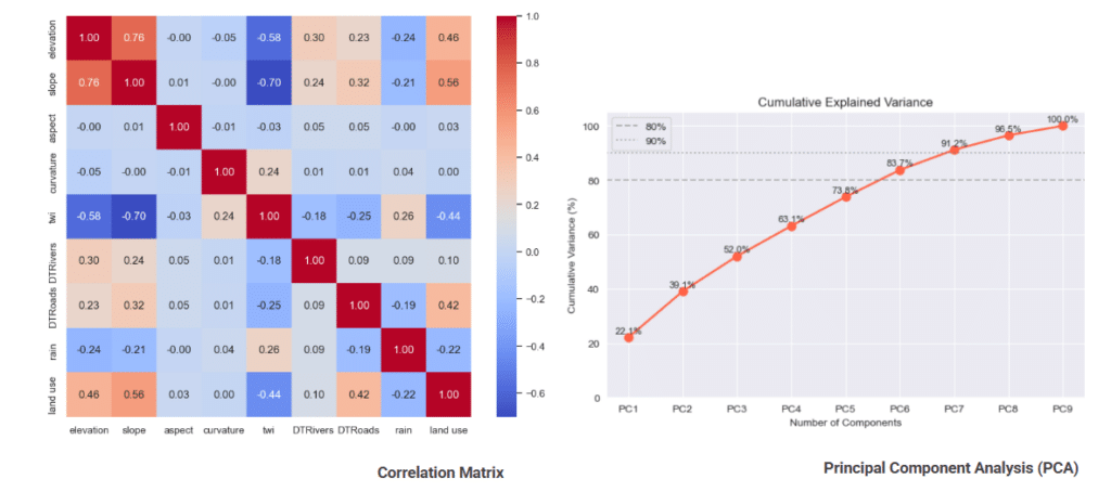
Then we checked for redundancy with a correlation matrix and PCA. Nothing’s a true duplicate — even our most related features carry their own information, and it still takes seven of the nine components to capture ninety percent of the variance.
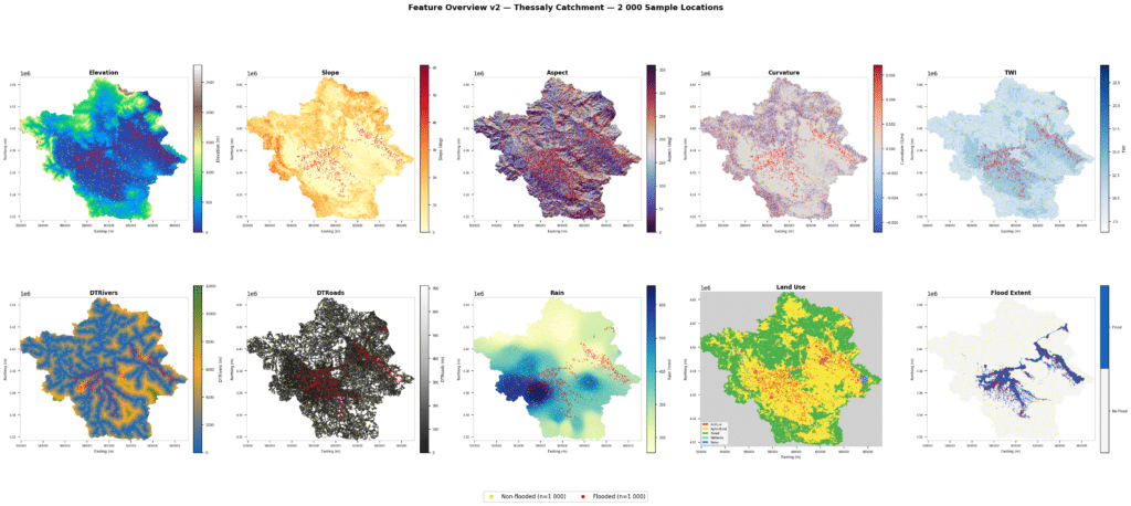
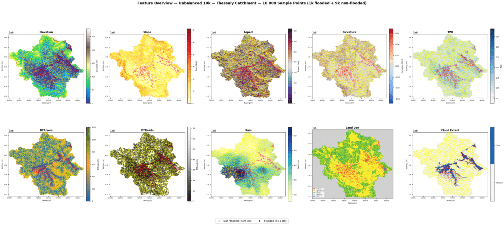
For better understanding of our features, we visualized the maps of all 9 features & flood extent across the Area of Interest.
Some conclusions before training:
Elevation & slope separate flooded from non-flooded most clearly, flooding concentrates on low, flat, water-collecting terrain.
Correlation matrix showed only elevation, slope, and TWI are moderately correlated. No two features are duplicates, so none can be dropped without losing information.
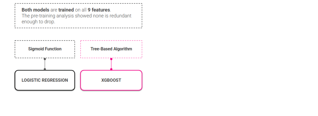
PCA showed the variance spreads across all components (7 of 9 needed for 90%), so the features can’t be compressed, so we proceeded with all 9 features.
The Two Models
We then trained two models: Logistic Regression and XGBoost that can pick up more complicated patterns.
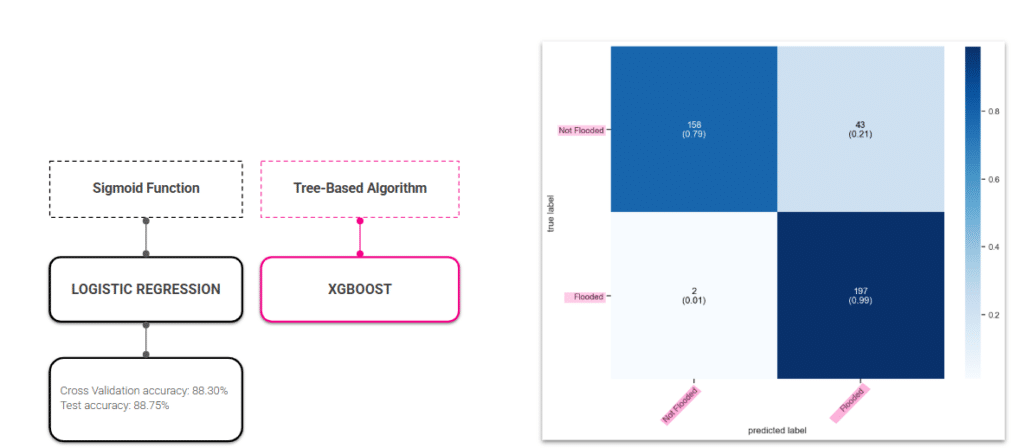
Logistic Regression (LR)
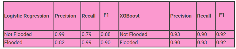
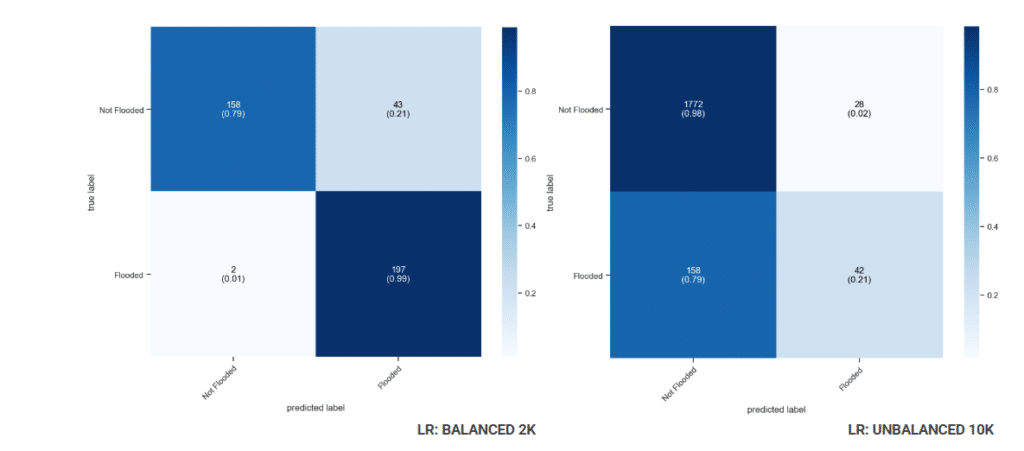
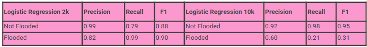
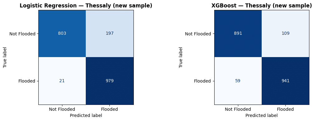
Logistic Regression reaches 88.75% test accuracy and correctly identifies 99% of flooded areas, missing only 2 out of 200, making it highly reliable at catching real flood events. The downside is 43 false alarms, where safe areas are incorrectly flagged as flood risk, a trade-off for being so sensitive to flooding.
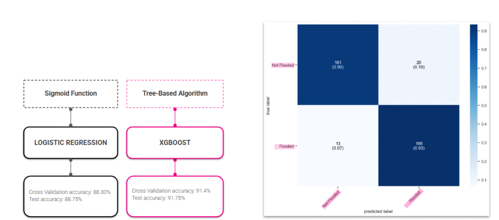
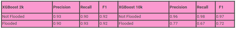
XGBoost reaches 91.75% test accuracy and correctly identifies 93% of flooded areas, while also being much better at avoiding false alarms, only 20 incorrect flood flags compared to LR’s 43. The trade-off is 13 missed floods, slightly more than LR’s 2, but overall XGBoost delivers a more balanced performance across both classes.
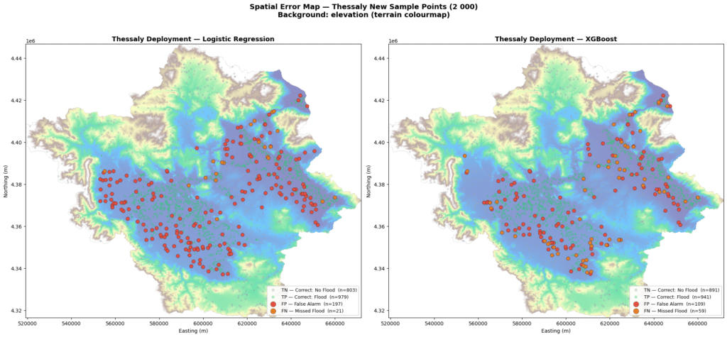
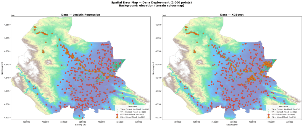
The 400 test set misclassifications can also be visualized on the map below.
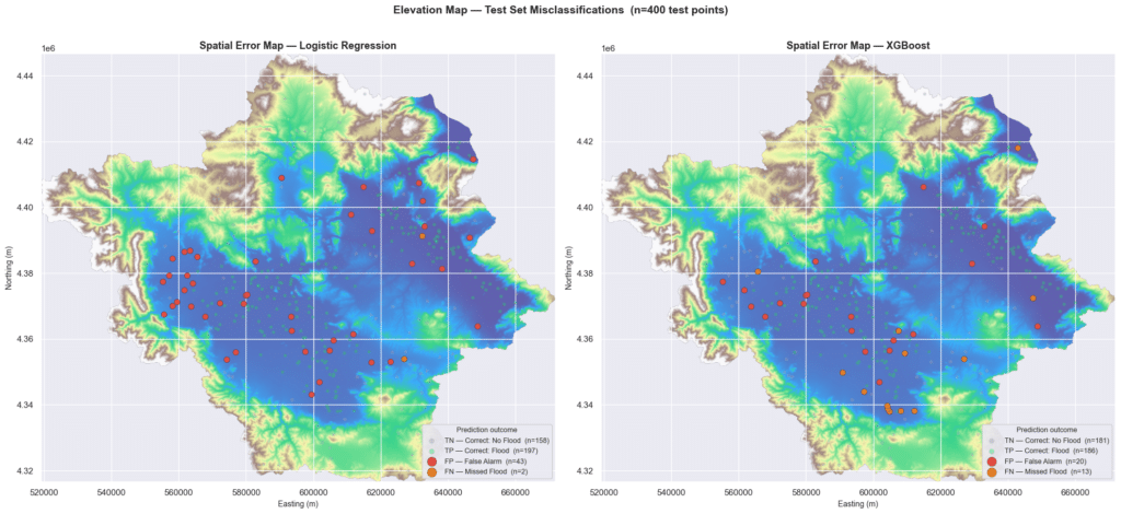
Both models struggle most in the flat central plain, where flood and non-flood areas share very similar terrain characteristics. XGBoost’s errors are fewer and more spread out, while LR tends to over-flag the lowlands, suggesting XGBoost draws a more precise flood boundary in areas where the terrain gives little away.
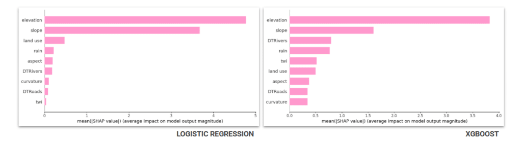
SHapley Additive exPlanations SHAP analysis confirms that elevation and slope dominate both models. Higher ground simply doesn’t flood, and steeper terrain drains faster. XGBoost captures non-linear relationships between features, which is why features like DTRivers, rain and TWI carry much more weight compared to LR.
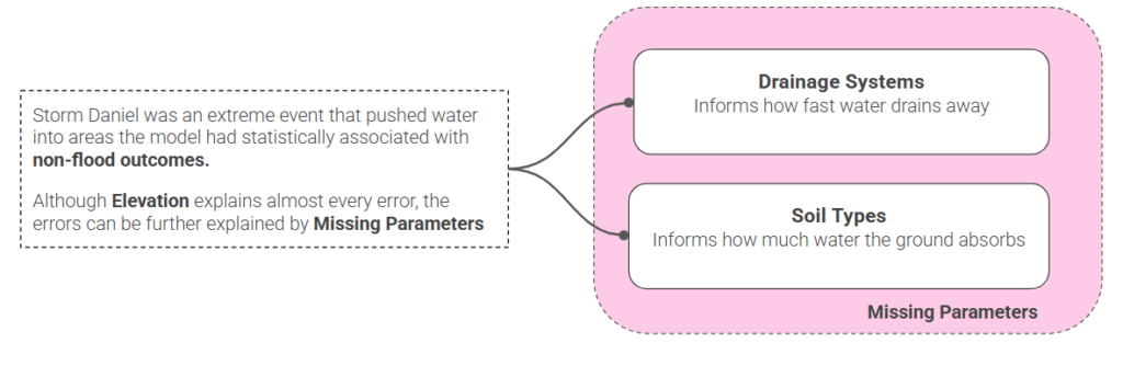
Almost every error is low, flat, agricultural land that looks like flood terrain but didn’t flood and we think it is because we’re missing two things the data doesn’t contain: drainage systems and soil type.
Reality Check
In reality, 90% of the Thessaly catchment is not flooded, so we built a 10k dataset that mirrors this 9,000 non-flooded and 1,000 flooded locations, to test how the models perform under real-world conditions.
The 10,000 sample locations plotted across all 9 features show the clear dominance of non-flooded points, with 9,000 yellow dots spreading across the full catchment and only 1,000 red flood points concentrated in the low-lying central plain near rivers.
When trained on unbalanced data, LR detects only 21% of real floods, missing 158 because the model is overwhelmed by non-flooded examples and learns to predict the majority class across the 2,000 test points.
When trained on unbalanced data, XGBoost detects only 67% of real floods , missing 66, a significant drop from 93% on the balanced dataset, showing that even the stronger model is badly hurt by the class imbalance.
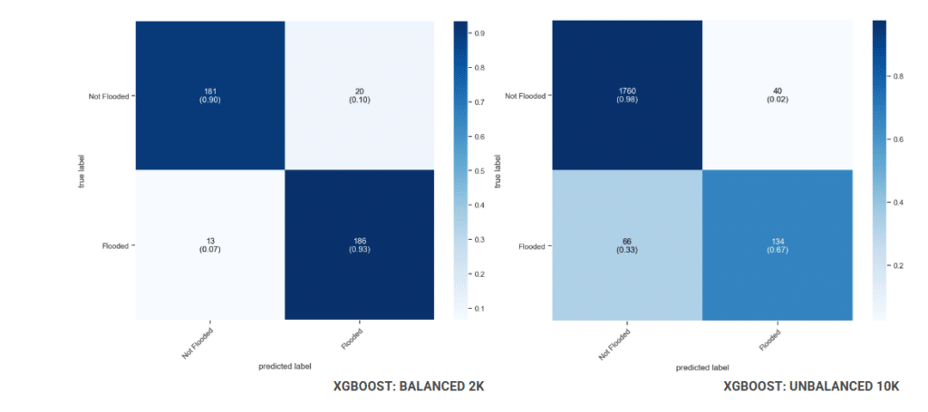
So we concluded that the balanced 2k dataset forces the model to learn the flooded class properly which justifies 1000/1000 samples as the right approach.
Deployment
First we deployed on unseen Thessaly points. The model holds, no degradation, honest performance. XGBoost produces fewer false alarms and fewer missed floods than LR on its own training ground.
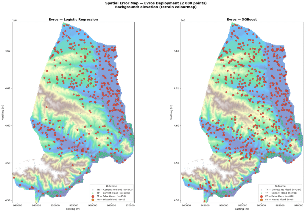
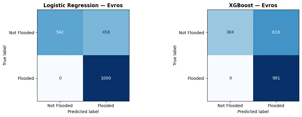
Then we deployed on a different region in the north of Greece, Evros.
Evros floods in February 2026 was not due to local rainfall. Snowmelt from Bulgaria and Turkey pushed the river over its banks for nine days. A riverine flood , completely different from Daniel. The feature maps immediately show how different this terrain is. Flat delta, narrow elevation range, slope nearly zero everywhere. Even rainfall is spatially uniform. The model is operating far outside what it was trained on.
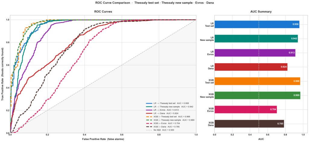
Logistic Regression holds at Area Under the Curve AUC 0.913. XGBoost collapses to 0.704 , barely above random. The simpler model travels better
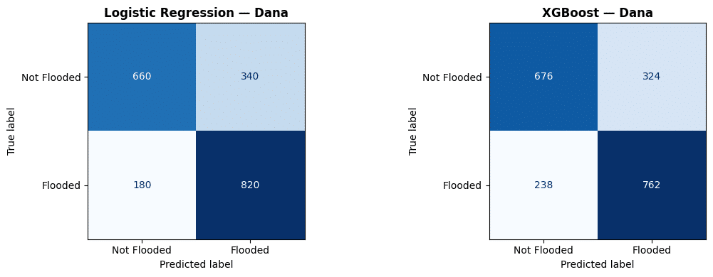
Finally, we tested on a different country, Spain. DANA flash flood (2024). The Dana terrain is more complex, elevated inland areas meeting a flat coastal plain, flood extent following river channels tightly. More variation in features but also more ambiguity for a model trained elsewhere.
Both models struggle more here. LR with AUC 0.82, XGBoost with AUC 0.79. Flash floods are driven by rainfall intensity in real time.
This chart below brings everything together in one view. Inside Thessaly both models perform comfortably, strong, reliable, as expected on home ground. Logistic Regression degrades gracefully as we move across regions 0.96 to 0.91 on Evros, down to 0.82 on Dana, losing ground with each step but never collapsing entirely. XGBoost tells a different story. It drops sharply on Evros , barely above random, before recovering slightly on Dana. The pattern is consistent: the more flexible model wins inside its training region and loses outside it.
Finally, we built and interactive map showing the full risk surface across all three regions. By clicking any point, all features and SHAP values will be shown for both models across all three deployment regions.
References:
Combining Machine Learning Models and Satellite Data of an Extreme Flood Event for Flood Susceptibility Mapping https://www.itia.ntua.gr/el/getfile/2562/1/documents/water-17-02678-v2.pdF
Post-Analysis of Daniel Extreme Flood Event in Thessaly, Central Greece: Practical Lessons and the Value of State-of-the-Art Water-Monitoring Networks https://www.itia.ntua.gr/en/getfile/2451/1/documents/water-16-00980.pdf
Copernicus Emergency Management Service (CEMS) – Storm Daniel 2023 Flood Maps
https://mapping.emergency.copernicus.eu
Greek Hellenic National Meteorological Service (HNMS) – Historical discharge & rainfall
https://emy.gr/en?area=forecast
GQIS/Open Topography