FABRICATED PROTOTYPES & DESIGN ANALYSIS
In this project, our group explored the integration of parametric modeling, robotic fabrication, and data-driven analysis to optimize clay-based 3D printing. We began by generating two vase geometries using Grasshopper and subsequently fabricated these designs with an ABB 120 robotic arm extruding clay. Throughout the process, we recorded both visual documentation and joint angle data extracted from RobotStudio. This dual approach allowed us to closely examine the relationship between robotic motion, print quality, and material performance.
Model 1
Data Collected
-Joint Angles (J1 to J6)
-Time Stamps
DESIGN ANALYSIS 1
The plot shows how the angles of each of the six joints of the ABB-120 robotic arm changed over time during printing process.
VELOCITY & ACCELERATION ANALYSIS
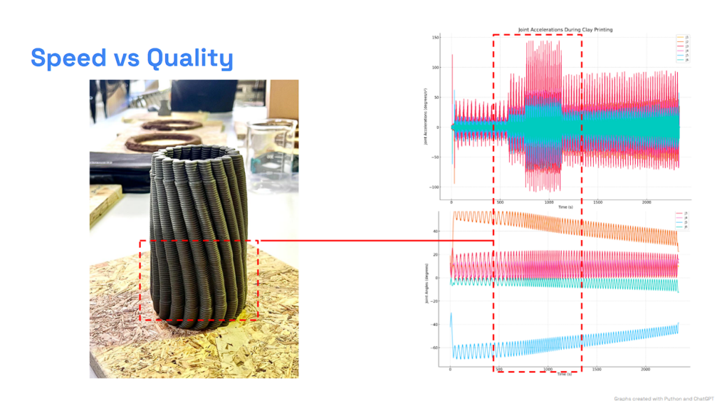
The plot illustrates the angular acceleration of each joint during the clay printing process. during the first printing process, we experimented with the speed of the printer output for the first model and the result of the process was mapped out in the graph on the right with each color on the graph mapping the axis on the printing arm. The analysis revealed several key issues. We observed how speed affects the print quality and graphs.
Calculation
Angular Velocity=Δ(Joint Angle)/ (Time)
Angular Acceleration=Δ(Angular Velocity)/Δ(Time)
Model 2
We intentionally experimented by changing the speed to understand printing process. The analysis revealed several key issues. We observed how speed affects the print quality and graphs. The shortcomings informed targeted adjustments for our second attempt, where we aimed to achieve an improved print quality. By analyzing the temporal joint angle data, we sought to correlate mechanical variables with observed setbacks in the fabrication process. This enabled us to identify patterns and potential areas for further optimization.
Data Collected
-Joint Angles (J1 to J6)
-Time Stamps
-Speed, Acceleration, Orientation
-End-Effector Position (only X-coordinate)
DESIGN ANALYSIS 2
The plot shows how the angles of each of the six joints of the ABB-120 robotic arm changed over time during printing process of the second vase model.
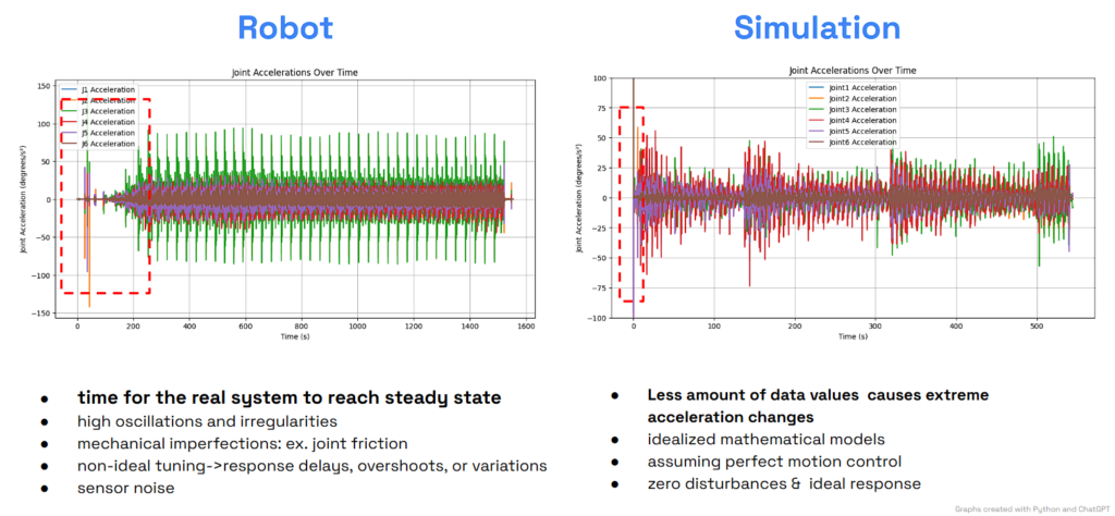
ANGULAR ACCELERATION
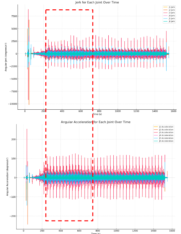
The first plot show the angular acceleration for each of the six joints (J1 to J6)
- Large spikes = sudden speed up or slow down
- affect -> smoothness of the process.
- acceleration should be smooth -> to prevent jolts
The second plot shows the jerk (Rate of Change of Acceleration) for each of the six joints (J1 to J6)
- jerk for each joint -> the rate of change of acceleration
- high jerk values -> quick change of joint acceleration
Calculation
Angular Velocity=Δ(Joint Angle)/ (Time)
Angular Acceleration=Δ(Angular Velocity)/Δ(Time)
Jerk=Δ(Angular Acceleration)/Δ(Time)
- The first plot depicts how the angular acceleration changes over time for each joint.
- Large spikes in acceleration indicate moments where the joint had to speed up or slow down suddenly, which can affect the smoothness of the printing process.
- Ideally, acceleration should be smooth to prevent jolts, especially during material deposition.
SPEED AND MAXIMUM LINEAR ACCELERATION of the END-EFFECTOR
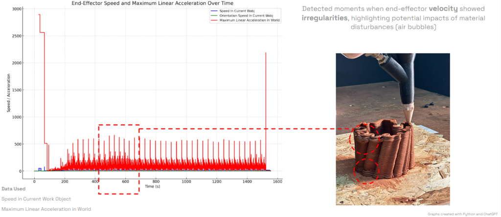
The spikes in the plot of speed and maximum linear acceleration of the end-effector during the printing of the second vase model can be indicative of several key issues or factors that affected the robotic arm’s movement. Here’s what those spikes could mean in the context of a clay printing process:
1. Material Flow Issues (ex. Air Bubbles)
- Air Bubble or Inconsistent Clay Flow: During the extrusion of clay, air bubbles can introduce inconsistencies, leading to sudden changes in the force needed to maintain the intended movement. This could cause the robot to react by either speeding up or adjusting abruptly, resulting in spikes in acceleration or speed.
- The spikes could correspond to the moments when the material flow was disturbed, and the robot had to compensate for that. For example, if there was a reduction in clay flow (due to an air pocket), the robot might accelerate to try to maintain the trajectory, resulting in spikes.
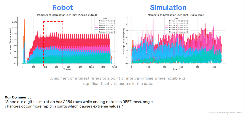
COMPARISON OF DATA EXTRACTED FROM ROBOT AND GRASSHOPPER SIMULATION
Potential Causes of Differences:
- Variations in data collection frequency:
- Data from Robot has 9657 rows
- Data from Simulation has 2964 rows
- Time difference
- Operational Conditions: Different payloads, speeds executed during the data collection.
- We didn’t print the whole geometry
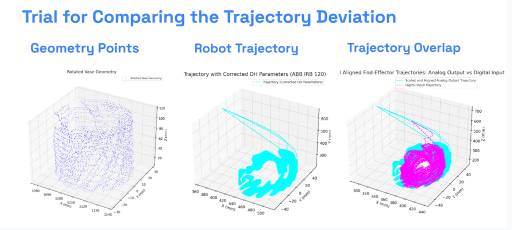
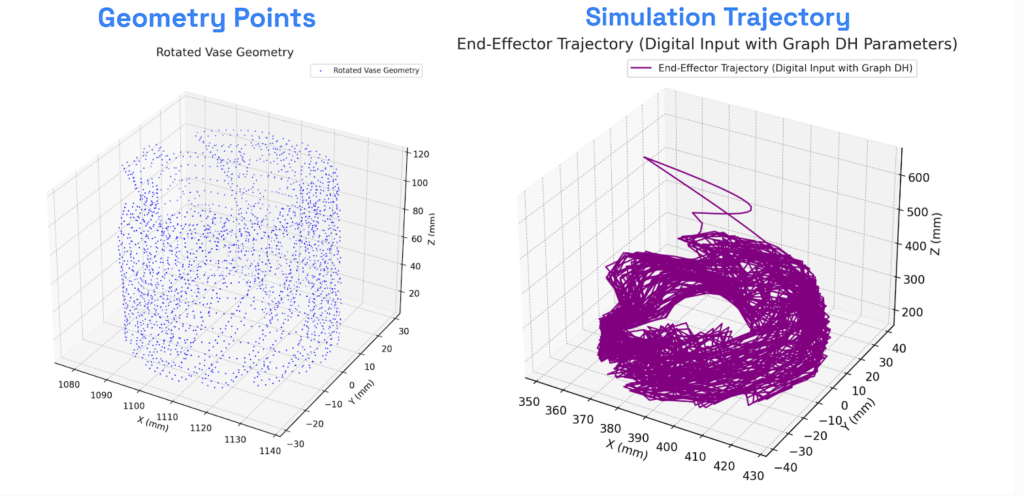
The plot compares the Joint Angle Graphs of ABB 120 Robot and Grasshopper Simulation
Subsequently, we compared the analog joint angle data collected during the physical printing with digital data obtained from a Grasshopper-based simulation. Although this comparison was complicated by discrepancies in speed and data resolution—2000 data points for the simulation versus 9000 for the actual print—it underscored the complexity of directly aligning digital predictions with physical outcomes.
JOINTS ACCELERATIONS
AI PROPOSALS
Predictive Quality Control:
- Anomaly Detection & Real-Time Alerts and Adjustments
Adaptive Path Planning:
- Use data to adjust trajectories in real time, reducing the impact of inconsistencies.
Generative Toolpath Design:
- Use GANs or deep learning to design optimized toolpaths to avoid inconsistencies.
AI-Driven Digital Twin for Process Optimization
- Leverage the collected data to create an AI-powered digital twin for real-time simulation and optimization of 3D printing processes.
Ultimately, these analyses highlight the potential of employing advanced data methods and AI-driven strategies to inform real-time adjustments in robotic printing, thus improving fabrication accuracy and overall performance.
MAPPING
THE INVISIBLE
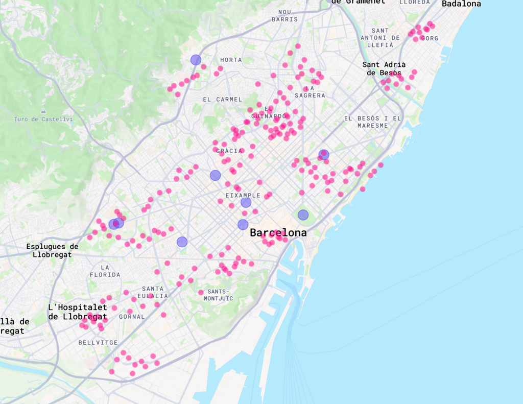
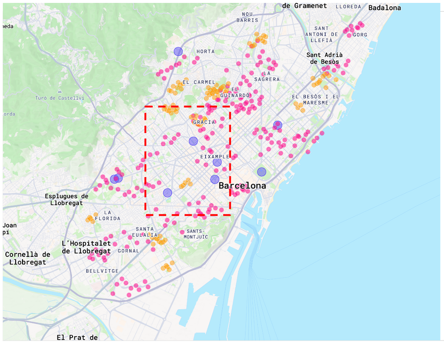
As cities like Barcelona strive to understand and respond to complex environmental challenges, the availability of detailed, city-wide climate data is essential. While a network of stationary IoT sensors can provide valuable snapshots of local air quality and microclimate conditions, each sensor only captures a small piece of the city’s environmental puzzle. Vast areas remain effectively “invisible”, limiting the precision and impact of policy decisions, urban planning, and community action.

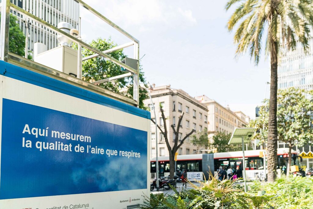
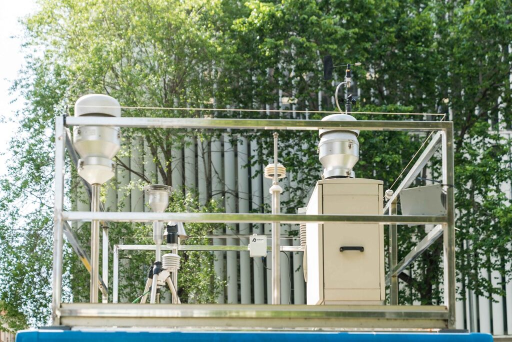
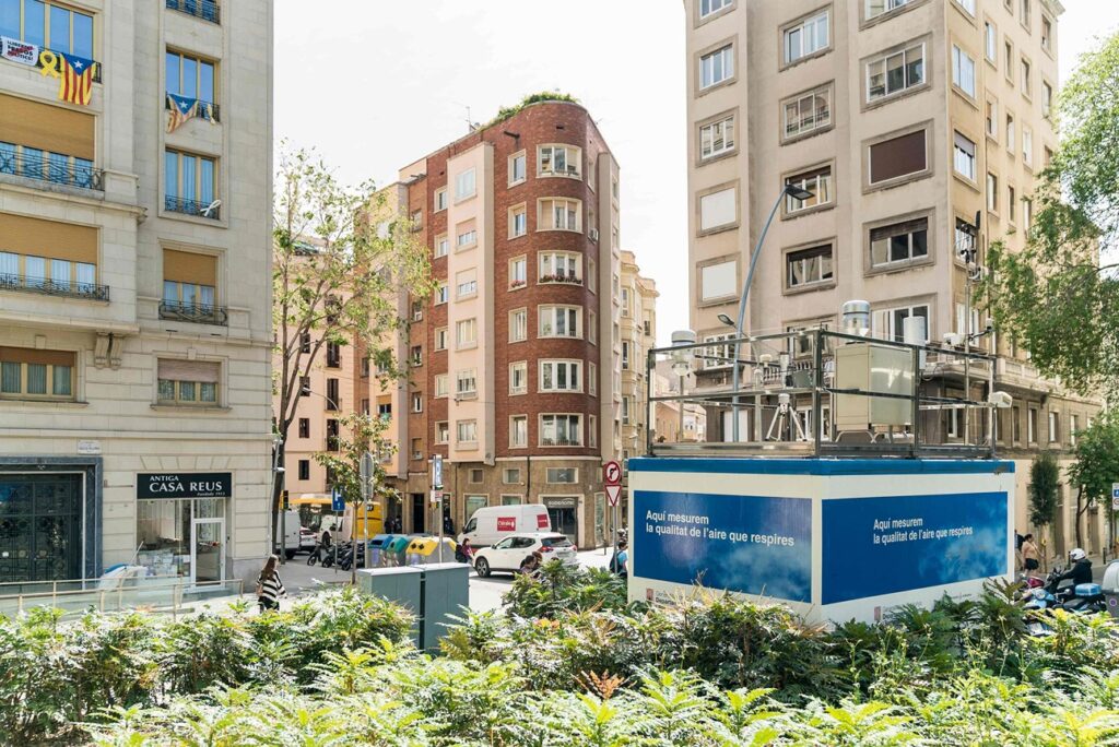
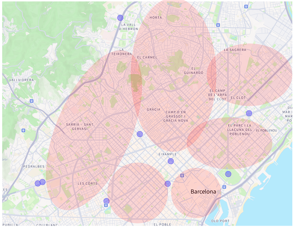
In Barcelona, 10 stations make up the Atmospheric Pollution Monitoring and Forecasting Network and they measure the air concentration of the main environmental pollutants that are harmful to people’s health. The data, along with other meteorological units and physical chemistry dispersion, is computer-processed and information on the pollutants in each area of the city is provided.
The stations monitor over 10 pollutants, including carbon monoxide, benzo[a]pyrene and heavy metals. It does not control the focus of the emissions, but it monitors the levels of concentration of pollutants in the air we breathe.The Atmospheric Pollution Monitoring and Forecasting Network is co-managed by the Government of Catalonia and the Barcelona Public Health Agency.
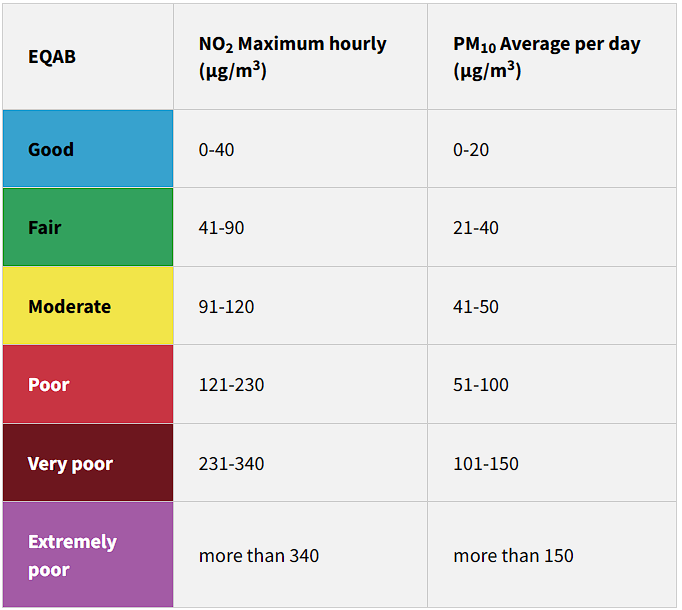
To facilitate the understanding of the level of Barcelona air quality in real time a six level classification has been established. These levels, represented with a colour code, range from good to extremely poor quality. Level scaling is based in Nitrogen Dioxide (NO2) and Particulate Matter (PM10) concentrations in the atmosphere.
The classification by levels is in accordance with the current definition of the Catalan Air Quality Index (ICQA)..
So in this project, we are going to build an ESP32 Air Quality Monitoring System using Nova PM SDS011 sensor, MQ-7 sensor, and DHT11 sensor. We will also be using an OLED Display module to display Air Quality Values. The Air Quality Index (AQI) in India is based on eight pollutants, PM10, PM2.5, SO2 and NO2, CO, Ozone, NH3, and Pb. However, it is not necessary to measure all of the pollutants. So we are going to measure the concentration of PM2.5, PM10, and Carbon Monoxide to calculate the Air Quality Index.
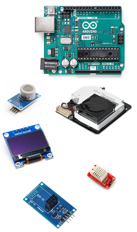
Components required | Real hardware setup
Wokwi Components | Simulation Setup
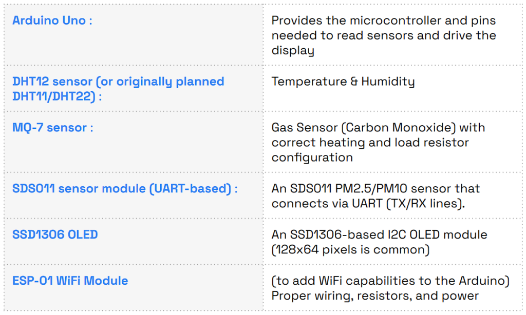
- Arduino Uno (Main) + Arduino Uno (Secondary as SDS011 mock) : Since Wokwi does not have the SDS011 dust sensor, we simulated the SDS011 by using another Arduino Uno board programmed to send SDS011-like data packets over serial (UART). This allowed the main Arduino to receive PM2.5 and PM10 readings as if a real SDS011 was connected.
- DHT12 (single-wire mode) instead of DHT22 : Initially, we wanted DHT11 or DHT22. Wokwi did not provide DHT11 or DHT22 in single-wire mode when requested, only a DHT12 with VCC, GND, SDA, and NC pins, which we used in single-wire mode (treating SDA as the data pin)
- Potentiometer instead of MQ-7 sensor : The MQ-7 sensor isn’t available in Wokwi. Instead of the actual CO sensor, a potentiometer module was used to provide a variable analog signal to the Arduino’s A0 pin, simulating changing gas concentration levels.
- Direct SSD1306 OLED component
- ESP-01 as WiFi Component: Wokwi supports ESP-01. We will add it and connect it to the Arduino’s serial pins.
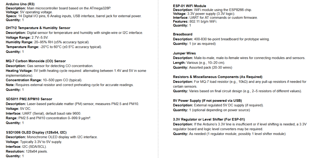
Bill of Materials (BOM) List components and their specifications.
Using this setup we place around 230 sensors which are equally distributed around the city of Barcelona and we can triangulate unknown data using regression models
