Quantifying the Opposite of Boredom
For decades, architectural design has relied on intuition. Client feedback and peer reviews are inherently subjective, and by the time you can gather real human response data on a facade, the building is already standing. But what if we could predict whether a building will be visually engaging before a single brick is laid?
Enter VenustaMeter, a machine learning project by Team Venusta (Zeynep Sezen Dursun, Marina Osmolovska, and Mahmoud Mohammad) for the MaCAD 2025/26 program. Deeply inspired by Thomas Heatherwick’s book Humanise, the project tackles Heatherwick’s crusade against “boring architecture”. While pure beauty might be too subjective to capture, VenustaMeter operates on a provocative thesis: boredom is actually measurable.
Ground Truth – Mathematical & Scientific Basis
The Science of Human Attention
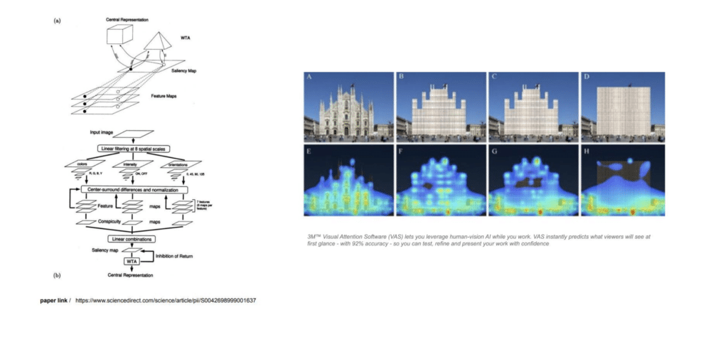
Itti, Koch & Niebur (1998) present a biologically-plausible computational model of primate visual attention. Multiscale image features — colour, intensity, and orientation — are filtered at eight spatial scales, combined into a single topographic saliency map, and a Winner-Take-All network sequentially selects the most conspicuous locations. The model breaks complex scene understanding into rapid, stimulus-driven attention shifts. Lavdas, Salingaros & Sussman (2021) demonstrated that 3M Visual Attention Software — built on Itti-Koch-Niebur — can predict implicit human engagement with building facades, showing traditional facades with nested symmetries score higher than minimalist contemporary ones. DOIbuildingbeauty
Workflow
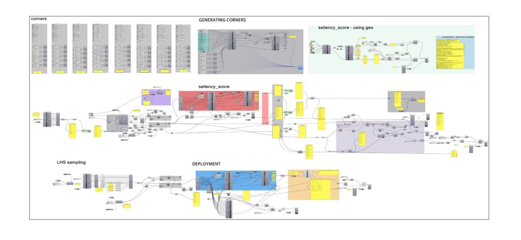
We designed a five-stage pipeline to extract, model, and deploy facade saliency intelligence — culminating in a real-time XGBoost predictor embedded natively within Grasshopper.
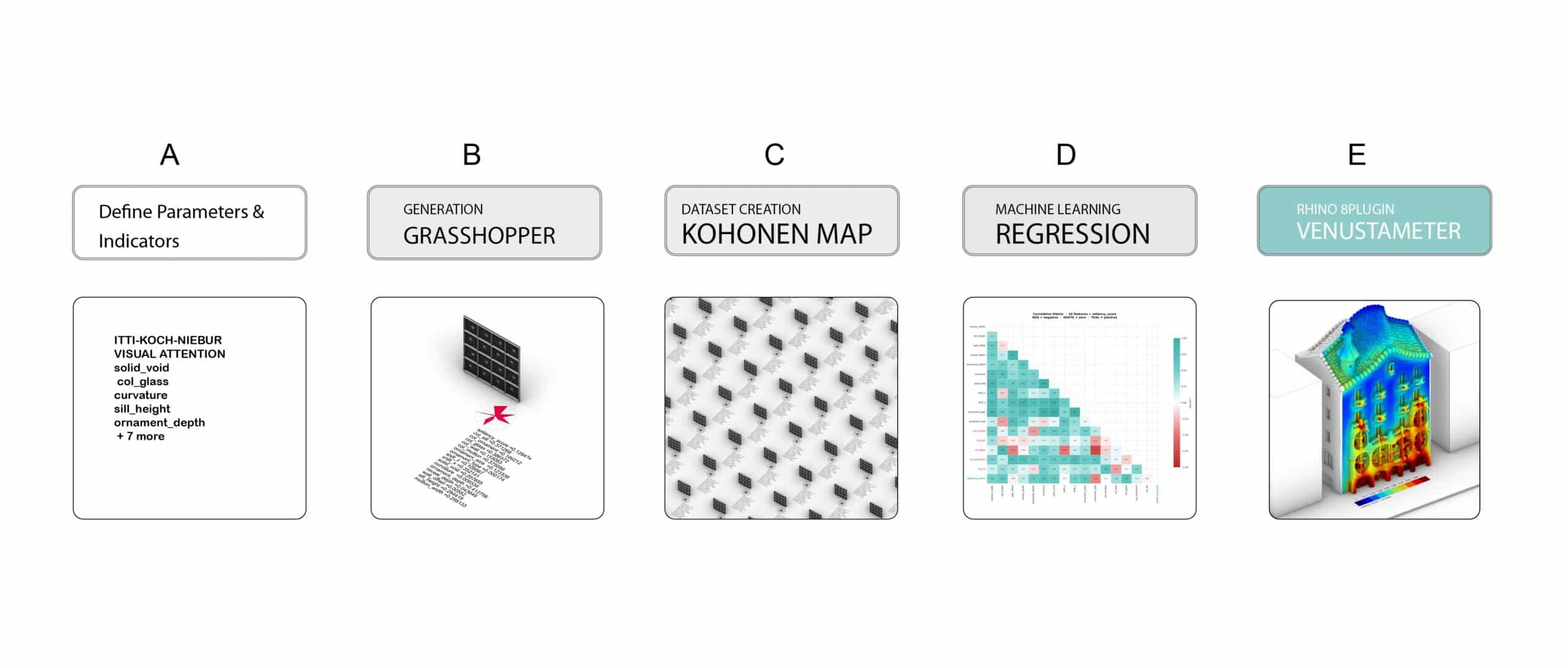
A |PARAMETERS & INDICATORS
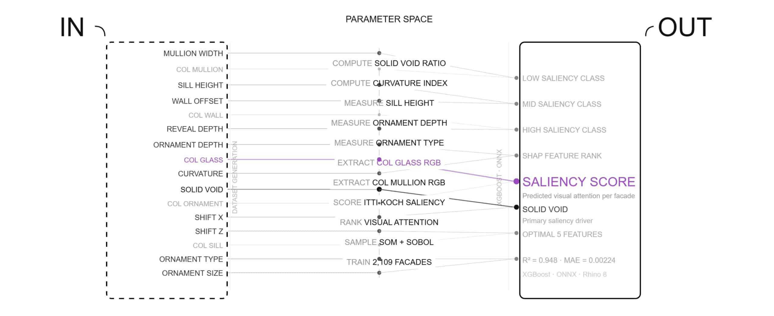
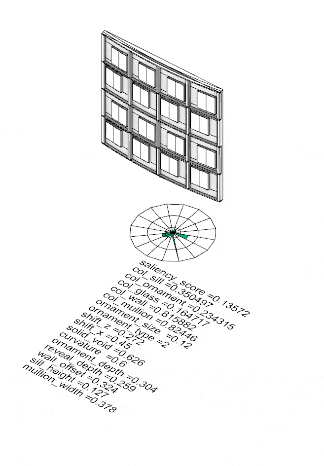
The first step grounds VenustaMeter in theory. We identified 16 measurable facade parameters — 11 geometric and 5 colour — drawn from the Itti-Koch-Niebur Visual Attention System. These define the input space fed into the Grasshopper definition, the computed parameter space processed through SOM sampling, and the saliency score output that the machine learning model learns to predict.
B | GEOMETRY GENERATION
With parameters defined, we built a Grasshopper definition that procedurally generates facade variants across the full 16-dimensional input space. Each variant is evaluated using the Itti-Koch-Niebur saliency algorithm to produce a ground-truth score. To ensure maximum diversity across the dataset, we applied NSGA-II multi-objective optimisation combined with SOM corner sampling — identifying the most extreme facade configurations across the parameter space as anchors for the Kohonen map.
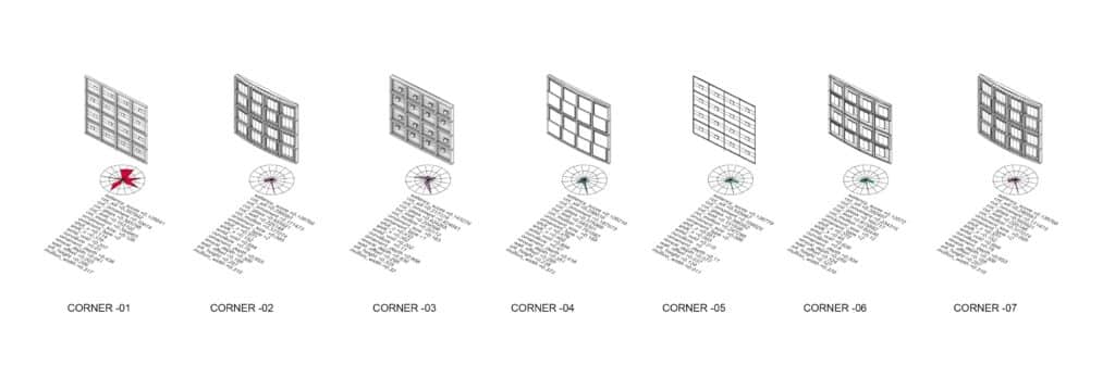
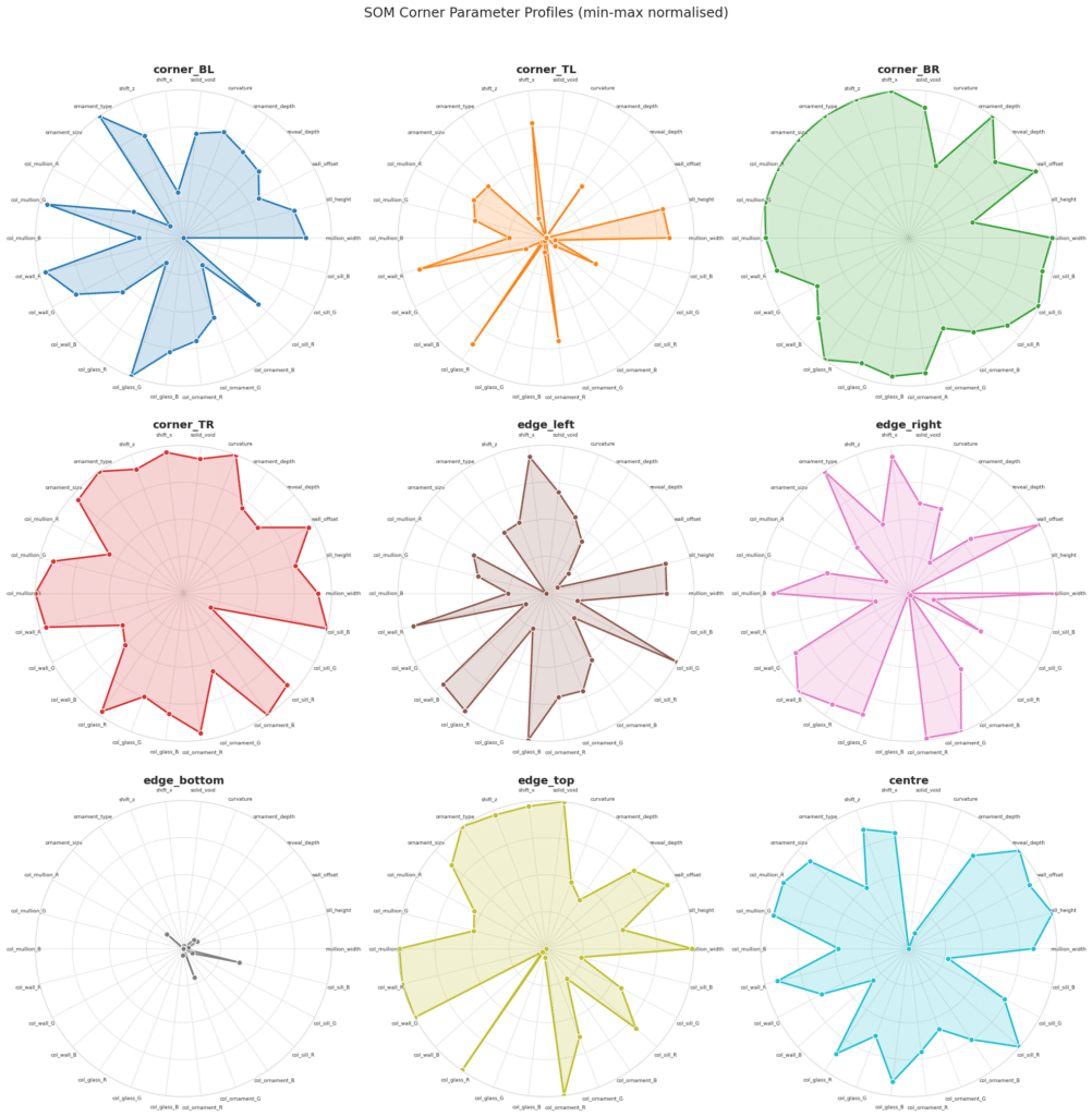
C | SOM + KOHONEN MAPS
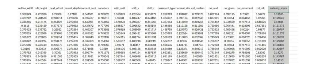
The four corner solutions from NSGA-II become seeds for something larger. Fed into a Kohonen Self-Organising Map, they propagate across a structured 45×45 grid — growing 2,109 facade variants that collectively span the full saliency landscape. On the left, the SOM distribution shows how samples spread across the parameter space; on the right, the resulting facade geometries. Every variant — its 16 input parameters and computed saliency score — is captured in facades.csv, the foundation on which the model is trained.
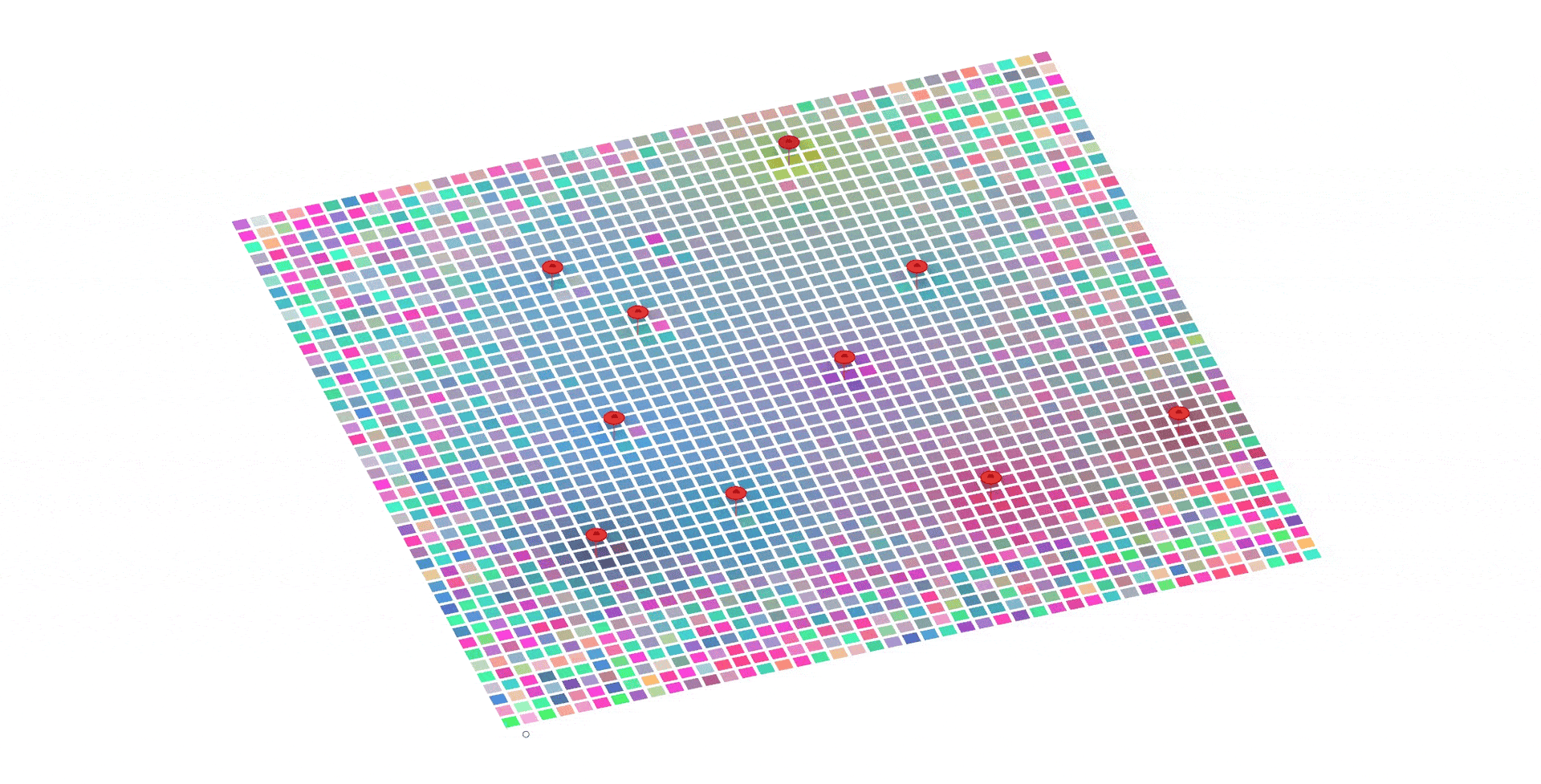
SOM map
spider chart
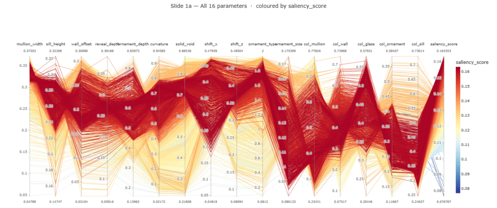
Parallel Coordinates — All 16 parameters
The plots confirm our features and dataset are sound: different parameter values map to different saliency outcomes. If a feature were irrelevant, its axis would show every saliency colour mixed at every height — no pattern. Instead, the geometry axes sort by colour (high-saliency lines bundle high on solid_void, curvature, ornament_depth, sill_height; low-saliency lines sit low), which means the saliency score genuinely responds to the parameters we chose. The variation is not random — so the dataset carries a learnable signal, and the features are the right ones to feed the model. The pattern is noisier in the 16-parameter plot and sharper in the geometry-only plot, because the colour parameters don’t separate saliency and removing them cleans up the signal — visual confirmation that geometry carries the saliency structure.
D | PCA + MACHINE LEARNING
Before training any model, we needed to understand what the data was telling us. Running a full PCA analysis across all 16 facade parameters revealed a clear geometry-led structure: PC1 and PC2 together capture 68.4% of total variance, with solid_void, curvature, and col_glass emerging as the dominant axes of saliency variation. This analysis guided our feature selection — reducing 16 inputs to the 5 that matter most.
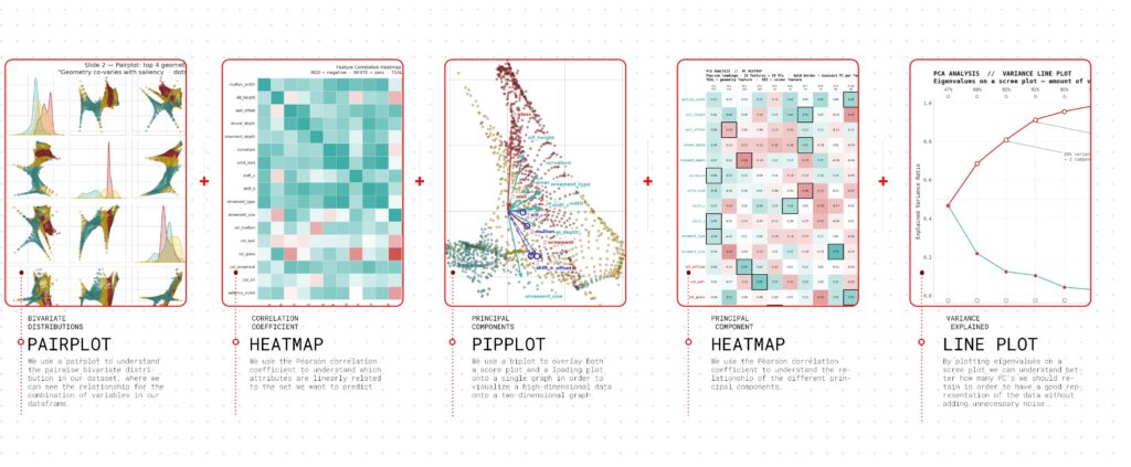
PCA ANALYSIS // PAIRPLOT
hese scatter plots establish our baseline. Before applying any complex model, we ran a simple Pearson correlation to prove that our geometric parameters actually influence the visual interest score. For instance, the strong upward trend in curvature proves that adding non-linear elements mathematically increases the facade’s saliency.
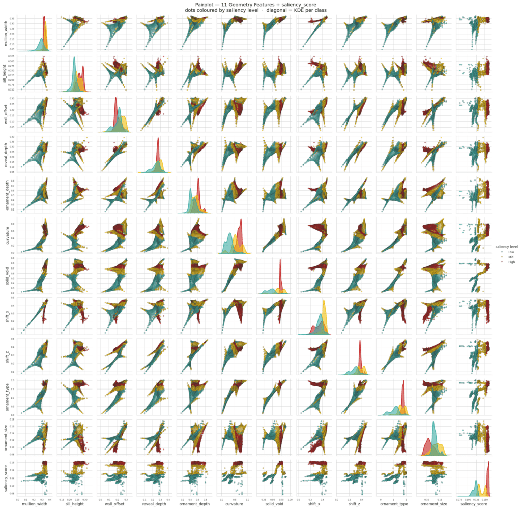
Correlation Heatmap
Feature Correlation Heatmap reveals which of the 16 facade parameters move together. ● Teal = positive correlation — geometry features cluster strongly together (solid_void, curvature, ornament_type move in sync) Red = negative — col_glass opposes several geometry features saliency_score row shows solid_void and curvature as strongest positive drivers
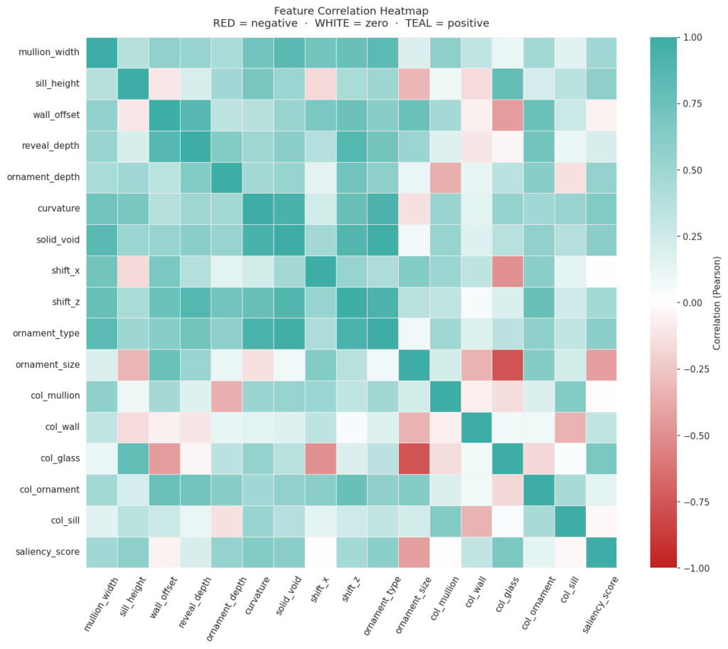
PCA ANALYSIS // PRINCIPAL COMPONENTS
This maps the DNA of our facades. The arrows show us the ‘pull’ of different features. Because the solid_void and mullion_width arrows stretch out so far along the X-axis, it proves that macro-geometry dictates the identity of a facade far more than surface color.
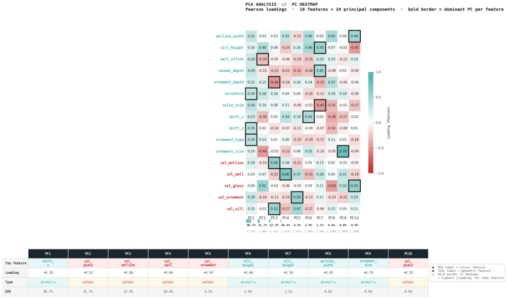
PC HEATMAP
Heatmap of PCA loadings — each of the 16 features against the first 10 principal components — with teal = geometry, red = colour, and a bold border marking each feature’s dominant PC; the table below names the top feature and explained-variance ratio (EVR) for each PC. The conclusion: variance separates cleanly into a large geometry axis and smaller colour axes. PC1 alone captures 47% of the variance and is geometry-driven (a broad bundle of solid_void, shift_z, ornament_type, curvature, mullion_width all loading together), while PC2–PC5 are led by colour features (col_glass, col_mullion, col_wall, col_ornament) — confirming geometry and colour vary along largely independent dimensions, with geometry carrying the bulk.
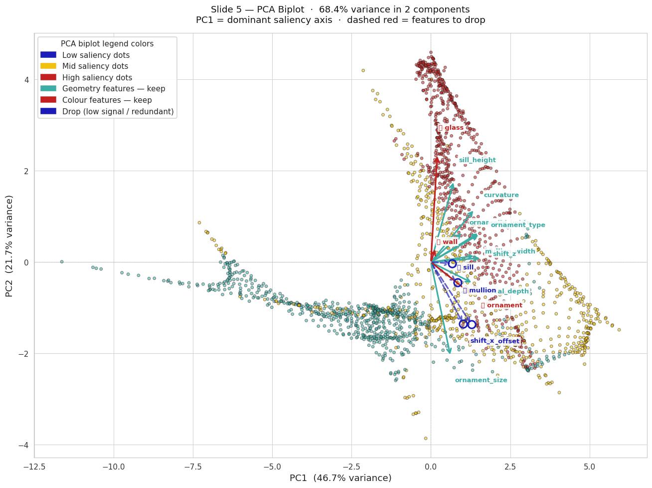
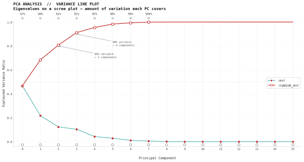
PCA-VARIANCE LINE PLOT
PCA Scree Plot shows how much information each Principal Component captures from the 16 facade features.Teal line (:evr) — each PC’s individual contribution, rapidly dropping after PC1Red line (:cumsum_evr) — running total: just 3 components capture 80% of all dataset variance, meaning most facade variation is explained by very few underlying patterns
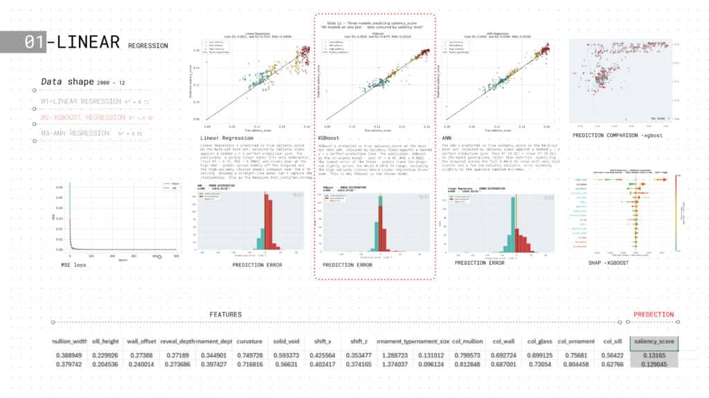
REGRESSION MODEL
Three regression models — Linear, XGBoost, and ANN — are compared on the same saliency prediction task. XGBoost leads with R²=0.95, ANN follows at R²=0.92, and Linear Regression trails at R²=0.72. SHAP values confirm solid_void and col_glass as dominant drivers. Prediction error distributions and residual plots validate XGBoost as the optimal model.
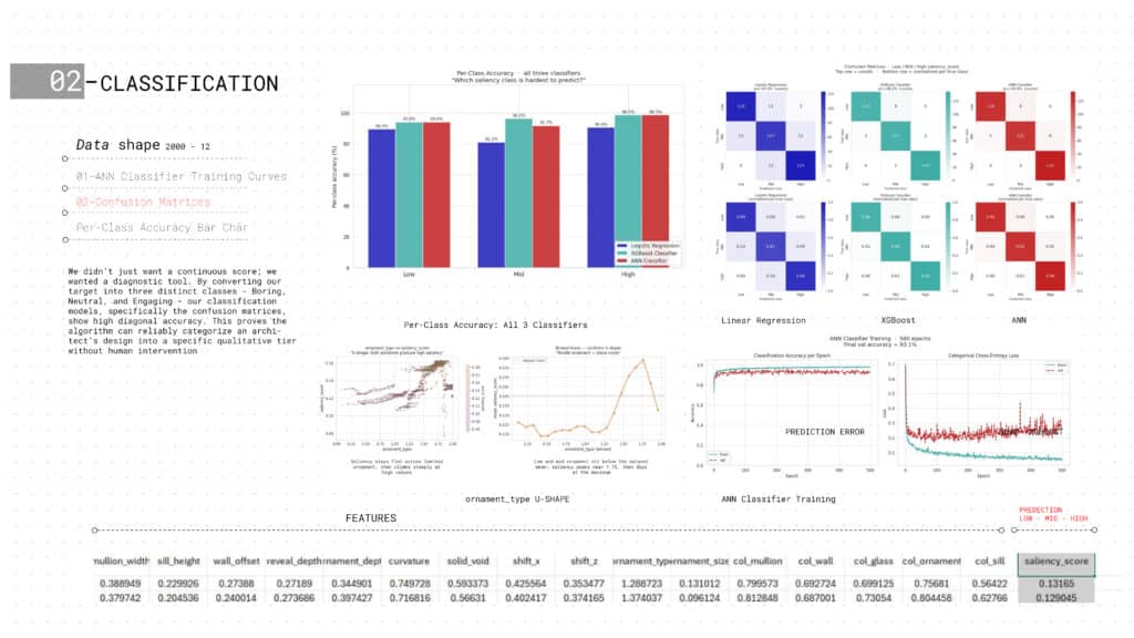
CLASSIFICATION MODELS
Beyond continuous prediction, VenustaMeter classifies every facade into three saliency tiers — Low, Mid, and High. XGBoost achieves 96.2% overall accuracy, ANN reaches 93.9%, and Logistic Regression 87.0%. Confusion matrices confirm near-perfect diagonal separation across all three classes. A key discovery: ornament_type follows a U-shaped relationship — extreme values at both ends produce high saliency, while mid-range ornamentation reads as visual noise.
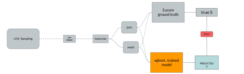
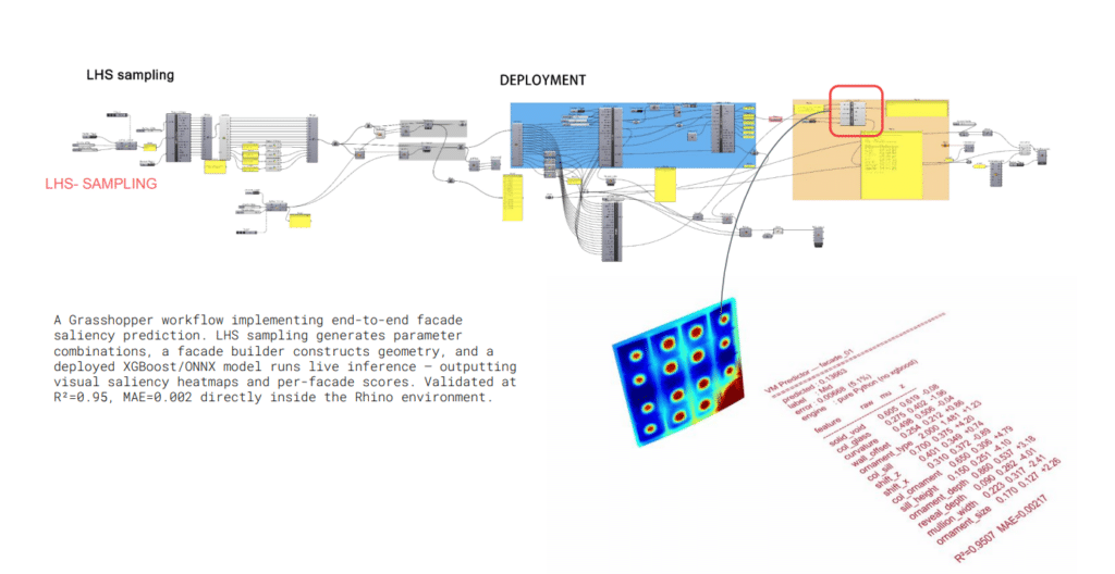
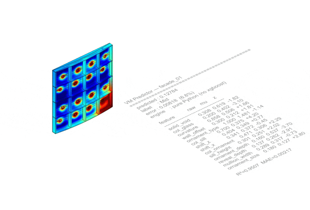
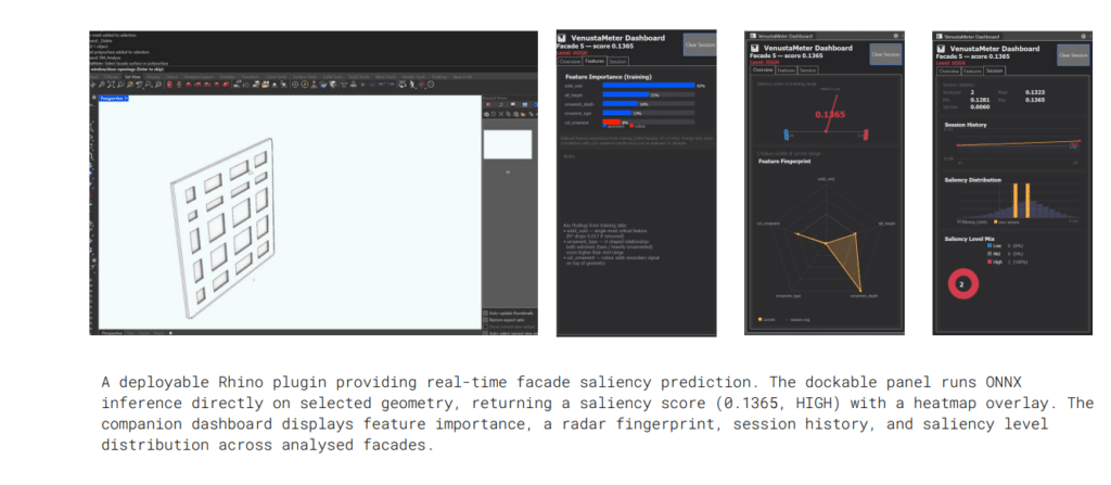
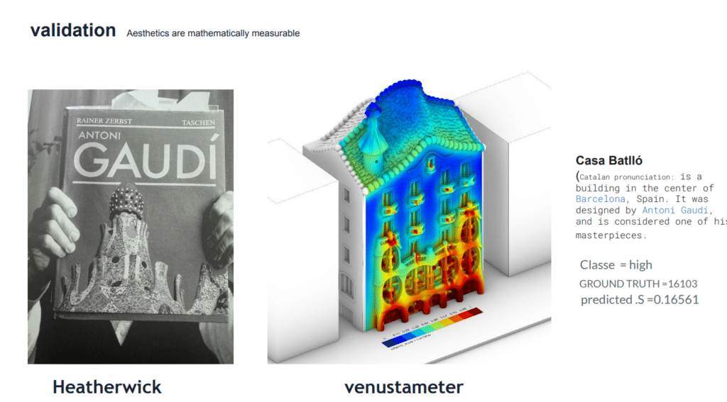
E |DEPLOYMENT
The trained XGBoost model is deployed natively inside Grasshopper via ONNX, enabling real-time saliency prediction without leaving Rhino. LHS sampling generates new unseen facade combinations — completely independent from the training dataset — and feeds them live through the pipeline. The model predicts saliency scores with R²=0.9507 and MAE=0.00217, confirming that accuracy holds on genuinely new data. Visual saliency heatmaps and per-facade scores output directly inside the Rhino environment.