The intent was to create a tangible, physical interface for real-time environmental simulation feedback in architectural design — letting designers manipulate physical building models by hand on a table, while a camera detects the arrangement and instantly projects live wind flow, solar exposure, or shadow analysis back onto the models. The goal was to remove the disconnect between physical model-making and digital simulation tools, so you could test a design’s environmental performance just by moving pieces around, instead of switching back and forth between physical maquette and CFD software.
Set Up
The physical setup is a tabletop pitched between a client and an architect standing on opposite sides:
- Overhead rig: a projector and depth camera mounted together above the table, both angled down to cover the model area (shown by the dashed cone).
- On the table: a 3D-printed base holding the site/building model, with LEGO massing blocks used to represent buildings that can be physically added or rearranged.
- How it works: the depth camera reads the physical arrangement of the model/LEGO pieces in real time, and the projector casts the simulation results (wind, sun, shadow, etc.) directly onto the table surface and models — so both people standing at the table see the environmental feedback update live as pieces are moved.
It’s essentially a shared physical workspace instrumented so that hands-on model manipulation and digital simulation happen in the same place at the same time, rather than the architect having to step away to a computer to run the analysis.

Wind Simulation Using Eddy 3D


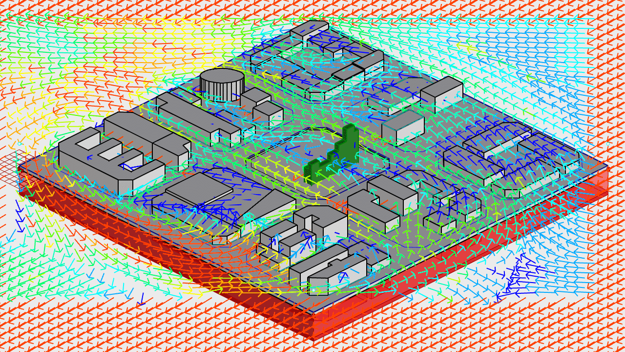
Section: Wind Simulation Using Eddy3D — explains the Grasshopper/Eddy3D workflow used to generate wind-flow visualizations over the site model. Two comparison images: a top-down wind simulation without a central building, and one with a building placed in the center, showing how the flow field changes around the added mass. A larger 3D projection render: the Grasshopper/Eddy3D wind simulation shown isometrically over the full massing model, with colored vector arrows indicating wind direction/speed across the site.
Web Socket for Projection Alignment
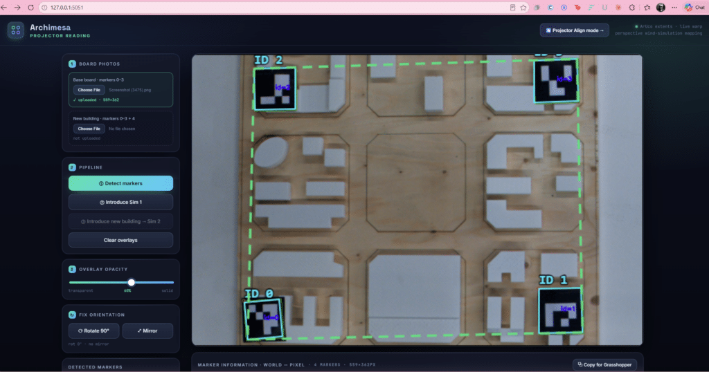
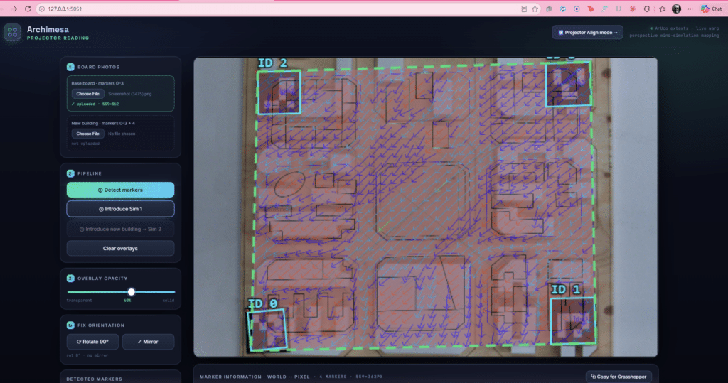
Base board uploaded: the 559×362px photo of the physical model on the table.
4 markers detected: IDs 0, 1, 2, 3 each get a cyan bounding box with their ID printed inside (you can see the actual black-and-white ArUco patterns clearly here since there’s no overlay yet).
Board extents locked: the dashed green rectangle traces the overall boundary formed by the four corner markers — this is the region that will later get warped and filled with the simulation overlay.
“Introduce Sim 1” is enabled but hasn’t been clicked yet — so the wind vector field hasn’t been projected on top. That’s why you’re seeing the clean, undistorted photo of the LEGO/foam massing model rather than the red-tinted vector overlay from the other screenshots.
New building slot still empty, so “Introduce new building → Sim 2” stays greyed out.
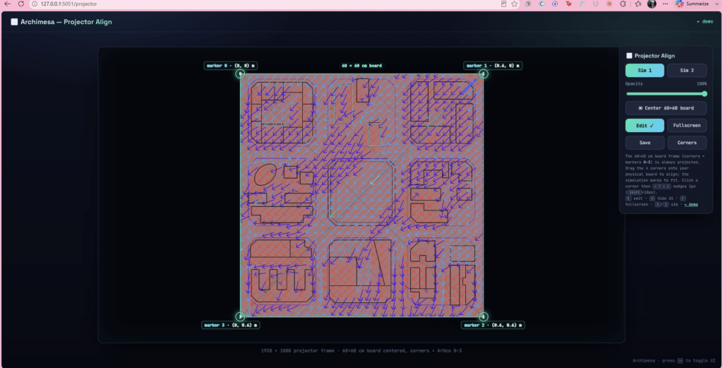
It projects a full-screen frame (1920×1080) representing the 60×60cm board, with the four corners labeled to match marker positions 0–3 at their real-world coordinates: marker 0 at (0,0), marker 1 at (0.6, 0), marker 2 at (0.6, 0.6), marker 3 at (0, 0.6).
The wind-simulation overlay (Sim 1, currently selected) is rendered inside that frame at 100% opacity.
The four corner handles (the small circular dots numbered 0–3) are draggable — you’re meant to physically point a real projector at the real board, then drag each corner handle until the projected frame’s corners line up exactly with the physical board’s corners. This corrects for keystone/perspective distortion from wherever the projector is actually mounted.
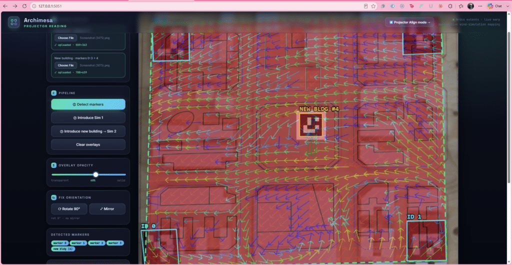
The base board photo (4 markers, IDs 0–3) has been uploaded and detected. Each marker gets an individual cyan bounding box with its ID labeled, and the overall board extent is traced with the dashed green rectangle. The wind vector field is already overlaid (Sim 1, the baseline simulation) at 60% opacity across the full board area. At this stage the “new building” upload slot is still empty, and “Introduce new building → Sim 2” is greyed out since it needs marker 4 present first.
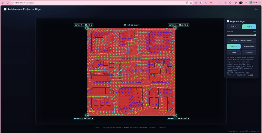
You can see the effect this has on the vector field: it’s noticeably different from Sim 1 — more yellow/green vectors flowing left-to-right and upward through the center-right of the board, versus Sim 1’s more uniform diagonal blue arrows. This is the re-solved wind field from after the new building (marker #4) was introduced, being projected in the aligned/calibrated view rather than over an uploaded photo.
Everything else on this screen works the same as the Sim 1 view: the corner handles at markers 0–3 let you drag to keystone-correct the projection against the physical board, Edit mode is active, and it’s still centered at 100% opacity within the 1920×1080 projector frame.
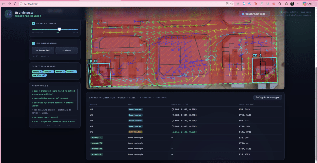
This is a scrolled-down view showing the underlying math behind the mapping: a table listing all 5 markers (0–4) plus the 4 board-extent corners, with each one’s real-world coordinates in meters (marker 0 at origin, marker 1 at 0.6m, etc., forming a 0.6×0.6m board) mapped to its detected pixel location in the photo. This is the homography data used to warp the simulation image onto the photo perspective correctly — you can see marker #4 (new building) sits at world position (0.016, 2.625, 0), notably outside the 0–0.6 board bounds, suggesting it’s a separate/floating marker rather than sitting flush on the board grid. The “Copy for Grasshopper” button suggests this table is meant to be exported back into your GH definition.