
Can Street Geometry Predict Urban Safety Risk?
A machine-learning pipeline that classifies street morphology into risk typologies — from OpenStreetMap features to multi-city deployment, dead ends included.
This post documents the full arc of our Urban Safety project — not just the results, but the reasoning, the wrong turns, and what we learned from them. The work traces a path from an ambitious question (can public spatial data predict crime?) to a more honest one (can it produce a coherent morphological typology of risk?). We think the second question is more useful to designers, and the path between them is worth showing.
00. Concept & Scientific Grounding
What are we predicting?
The core question is whether street geometry — measurable from public map data — can predict urban safety risk. We framed it as a three-class problem: low, medium, or high risk, using spatial features drawn from OpenStreetMap and secondary sources.
To be precise about scope: we are not predicting crime, and we are not measuring how safe people feel. We are asking whether the physical layout of a street alone gives us enough signal to group street segments into meaningful types.
Grounding in sixty years of urban safety theory
Each feature in our pipeline is anchored in established theory. Jane Jacobs argued that active entrances create natural surveillance — “eyes on the street.” Oscar Newman showed that territorial clarity reduces the conditions for risk. Bill Hillier and Julienne Hanson demonstrated through Space Syntax that network configuration shapes movement patterns in predictable ways. Every feature we chose can be traced back to at least one of these lineages.
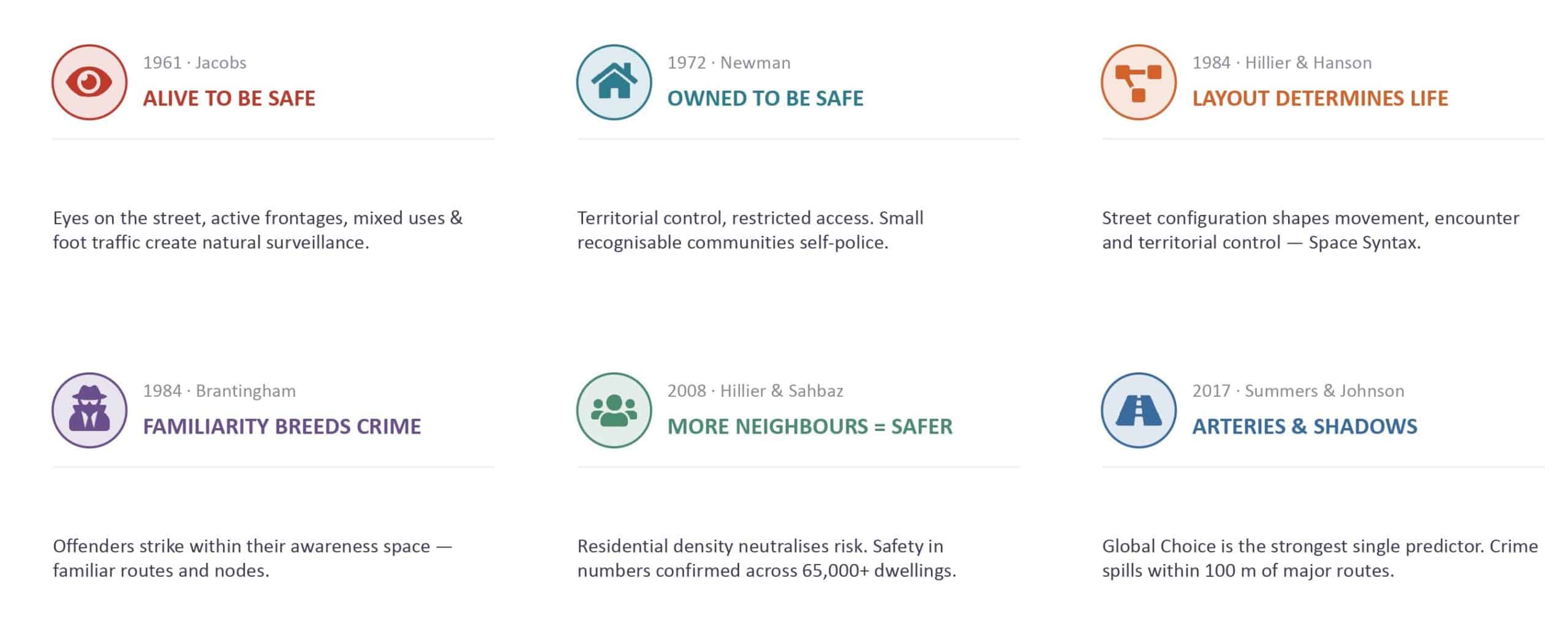
"The strongest pushback comes from Sampson, Raudenbush, and Earls (1997): the biggest predictor of neighbourhood violence is collective efficacy — whether residents are willing to intervene. We don't disagree. But spatial form is the lever designers can actually pull. You can't design collective efficacy, but you can design a street."
01. Initial Framework & Hitting a Wall
Classification over regression
In supervised machine learning, classification and regression are the two fundamental task types, distinguished by the nature of their output.
Classification predicts a discrete category or label — for example, determining whether an email is spam or not, or identifying which digit appears in an image. The model learns a decision boundary that maps inputs to one of a finite set of classes.
Regression, on the other hand, predicts a continuous numerical value — such as estimating a house’s price, forecasting tomorrow’s temperature, or predicting a user’s age. The model learns a function that maps inputs to a point on the real number line.
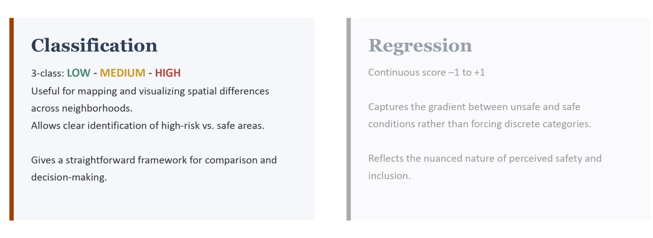
We chose classification over regression deliberately. A continuous score might capture more nuance, but three categories — low, medium, high — are immediately readable on a map and actionable for design. The output has to be usable.
Unit of analysis: the street segment
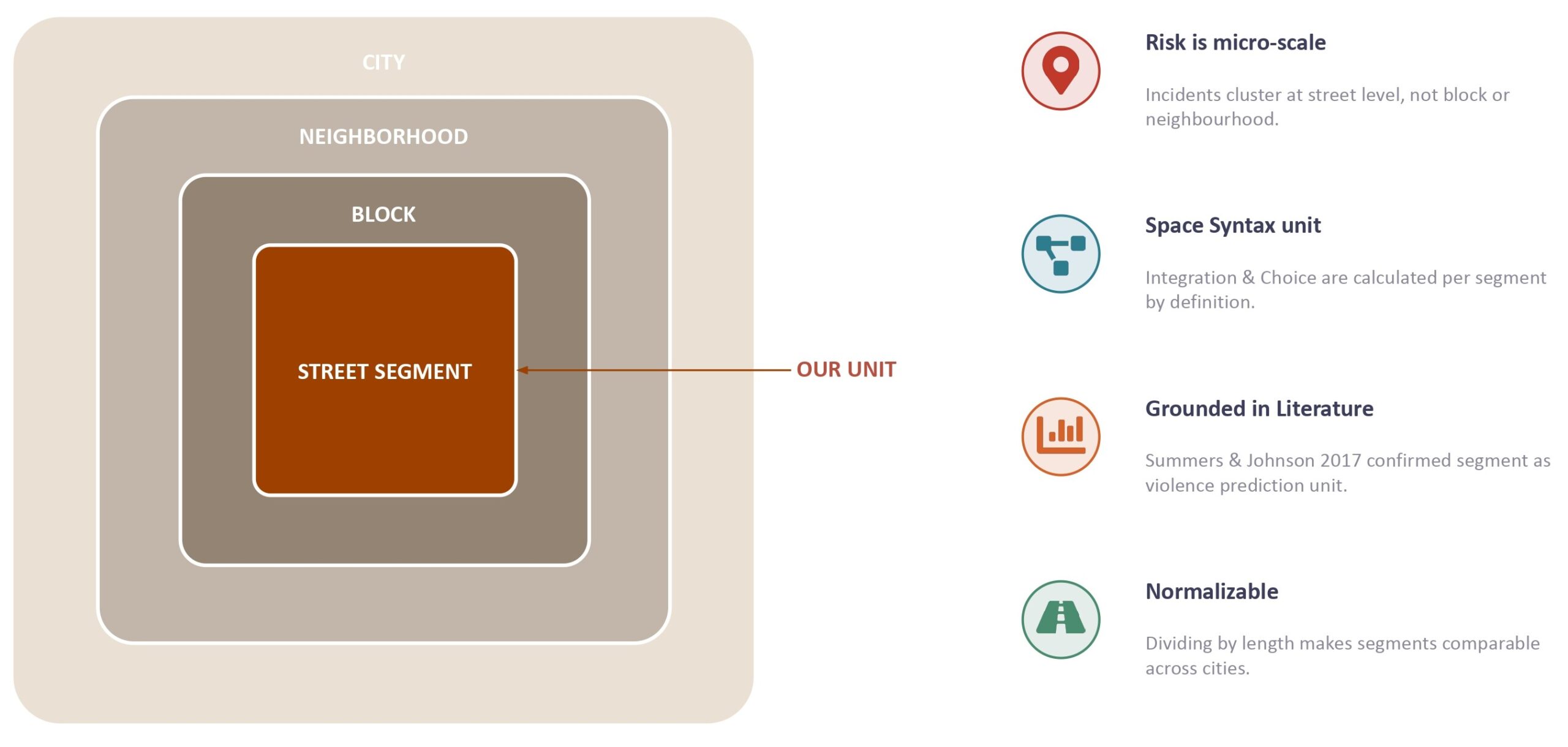
Our unit of analysis is the stretch of street between two intersections. Four reasons: risk clusters at that scale; Space Syntax operates segment by segment by definition; segments can be length-normalized; and a classified segment points a designer to a specific, addressable piece of street.
02. Crime Data Mindset
Initial setup: can spatial features forecast crime?
With features and unit of analysis established, we initially aimed to test whether our spatial features could forecast crime on individual streets. We built a linear regression formula with four features — lighting, visibility, connectivity, and enclosure — assigning weights based on existing literature.
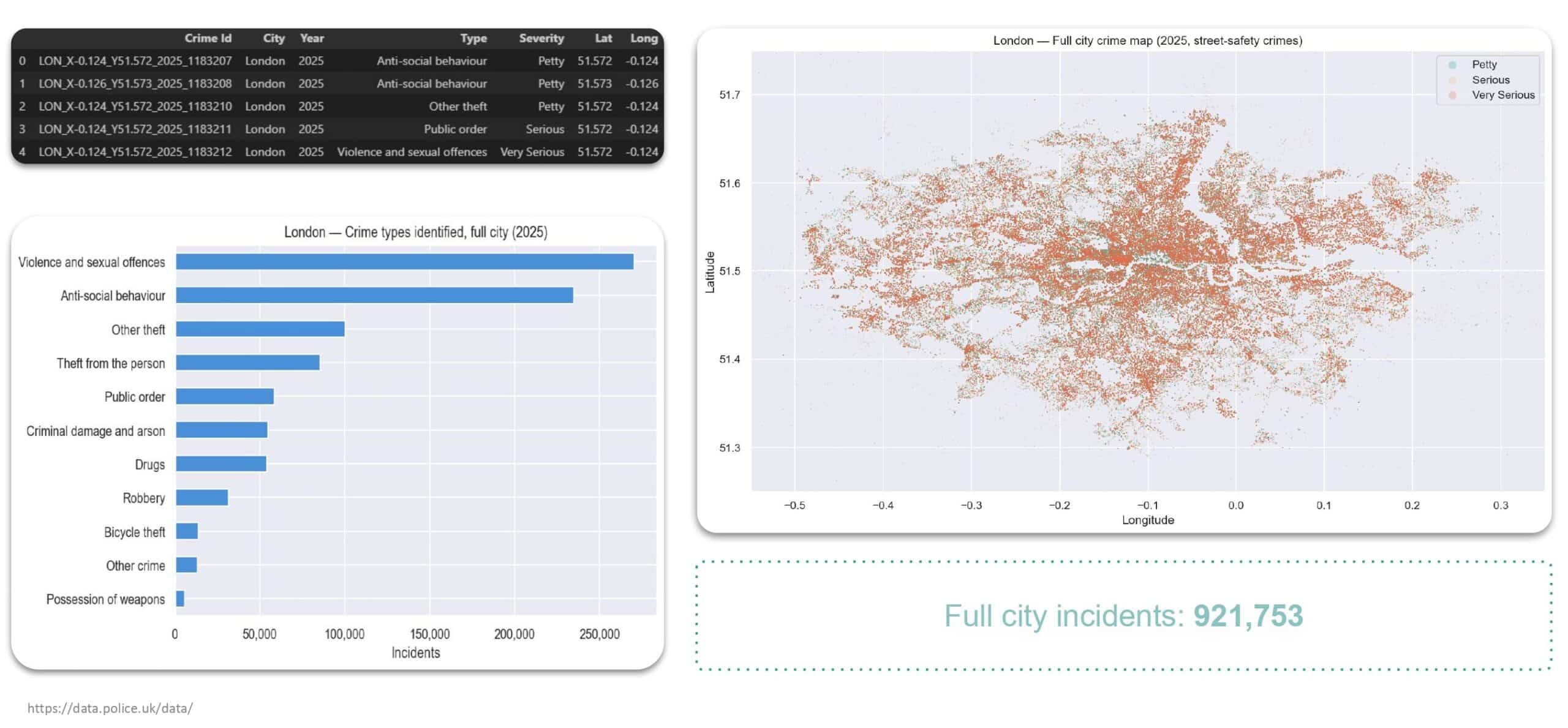
For the target variable, we sourced 2025 crime data for London covering approximately 920,000 incidents, classified into three severity tiers. Spatial mapping shows that while crime spans the entire urban area, it concentrates most densely in inner London.
London: Five boroughs, 36,000 segments
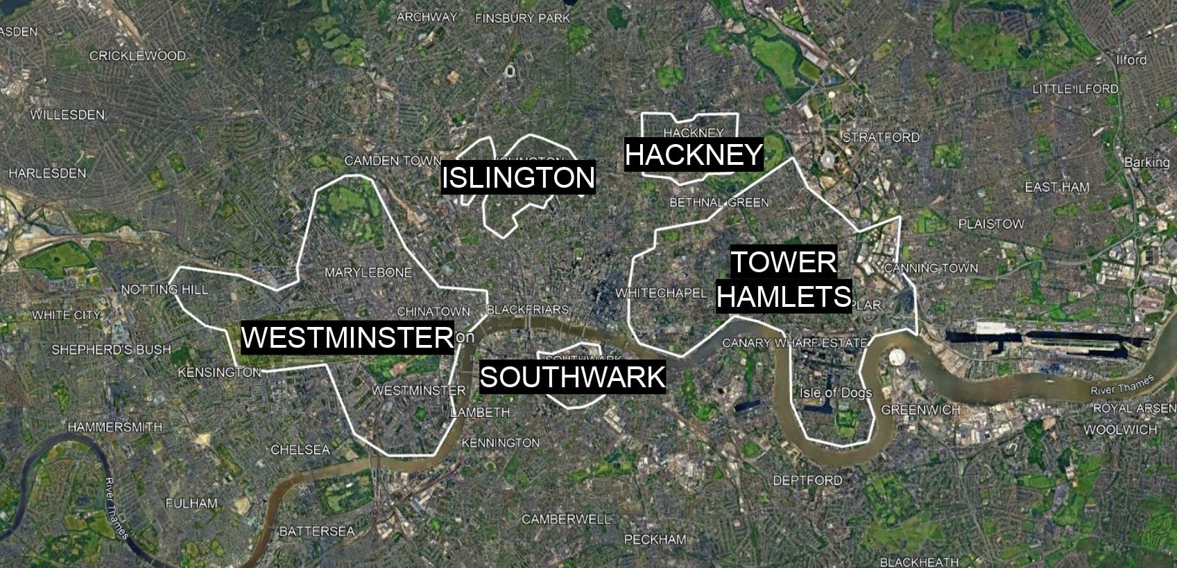
We extended the study beyond Islington to five boroughs chosen to represent a range of London’s urban morphologies — covering over 36,000 street segments in total. Before running any models, we performed a manual sanity check — cross-referencing our highest-risk street segments in Islington with Google Earth imagery to verify that features reflected real-world conditions.
The wall
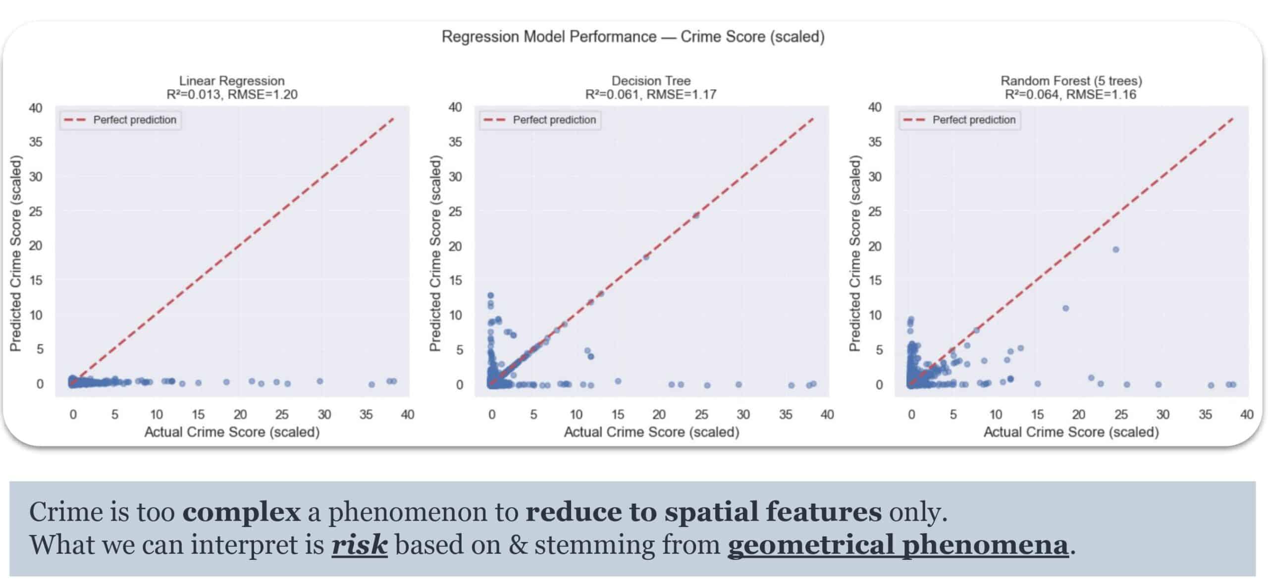
Three models — Linear Regression, Decision Tree, Random Forest — all yielded R² values under 0.064. The models failed to learn.
Crime is driven by complex social and economic factors that spatial features alone cannot capture.
We treated this as a finding rather than a failure. Since spatial features are too weak for direct regression against crime, we pivoted to a more honest goal: building a spatial typology that serves as a proxy for perceived risk.
03. Risk Assessment Mindset
The pivot
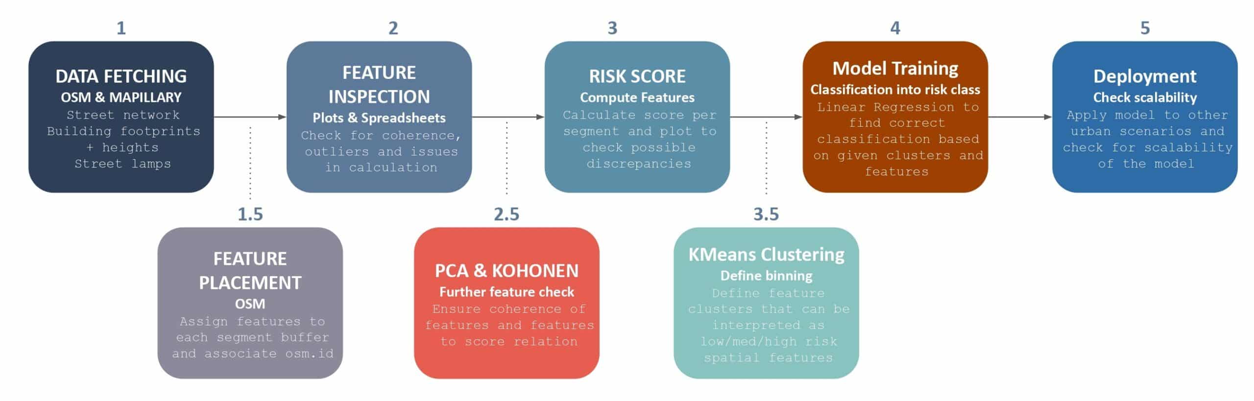
After the pivot, we rebuilt the pipeline into eight steps: fetch from OSM and Mapillary; place features onto each segment; inspect them; collapse into one risk score; use PCA and a Kohonen map as diagnostics; cut into three classes with K-Means; train the classifier; deploy to other cities. That last step is the real question — will it scale?
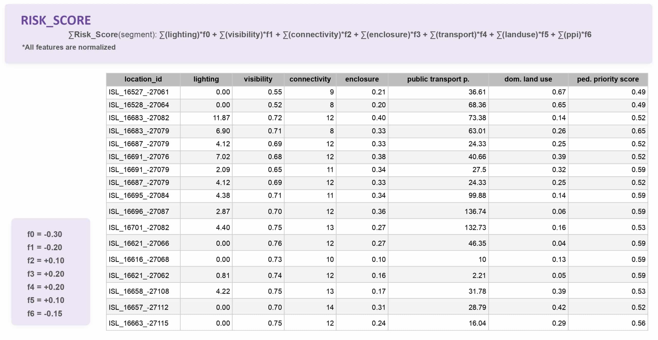
We extended the feature set with land-use mix and transit-stop proximity (both reliably in OSM), then added a seventh: the Pedestrian Priority Score from sidewalks, cycleways, and speed zones. This is not measured foot traffic — it shows whether a street is designed for pedestrians.
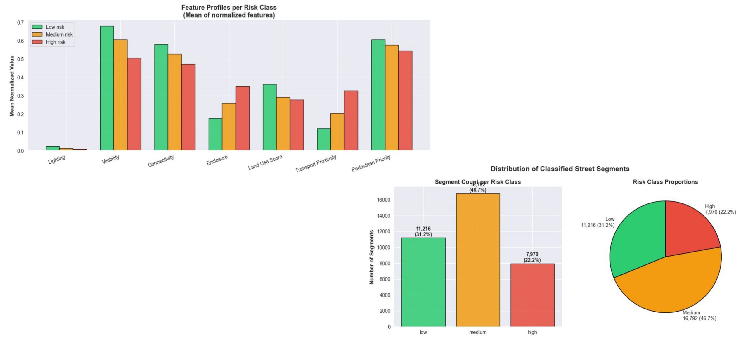
Resulting dataset
Each row is a segment with seven normalised features. The risk score is a weighted combination — safety factors pull it down, risk factors push it up. The weights come from the literature, not the data. An honest limitation.
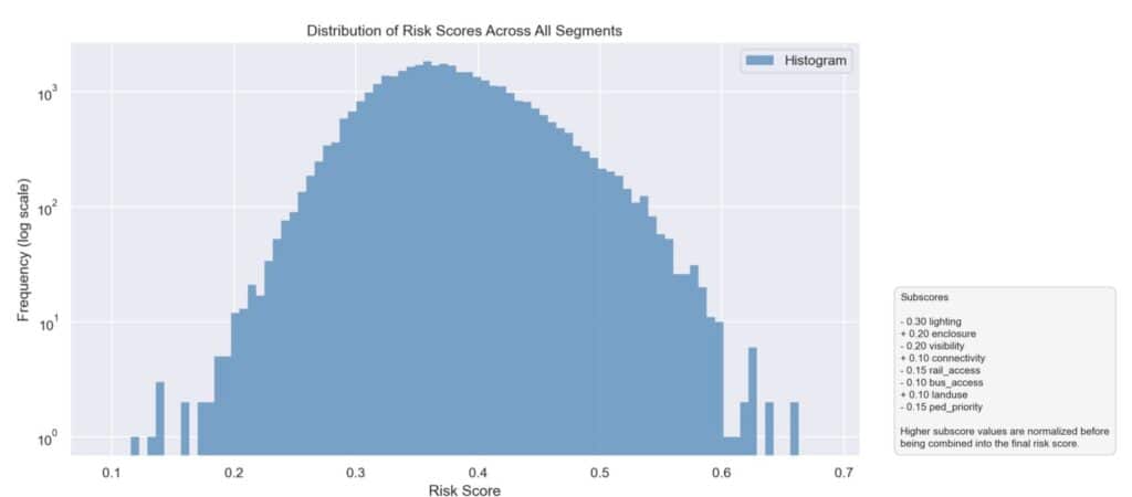
Across 36,000 segments, the score is roughly normal, centred near 0.35. Fixed cuts at 0.33 and 0.66 would slice through the densest part — so we let K-Means find the natural breakpoints.
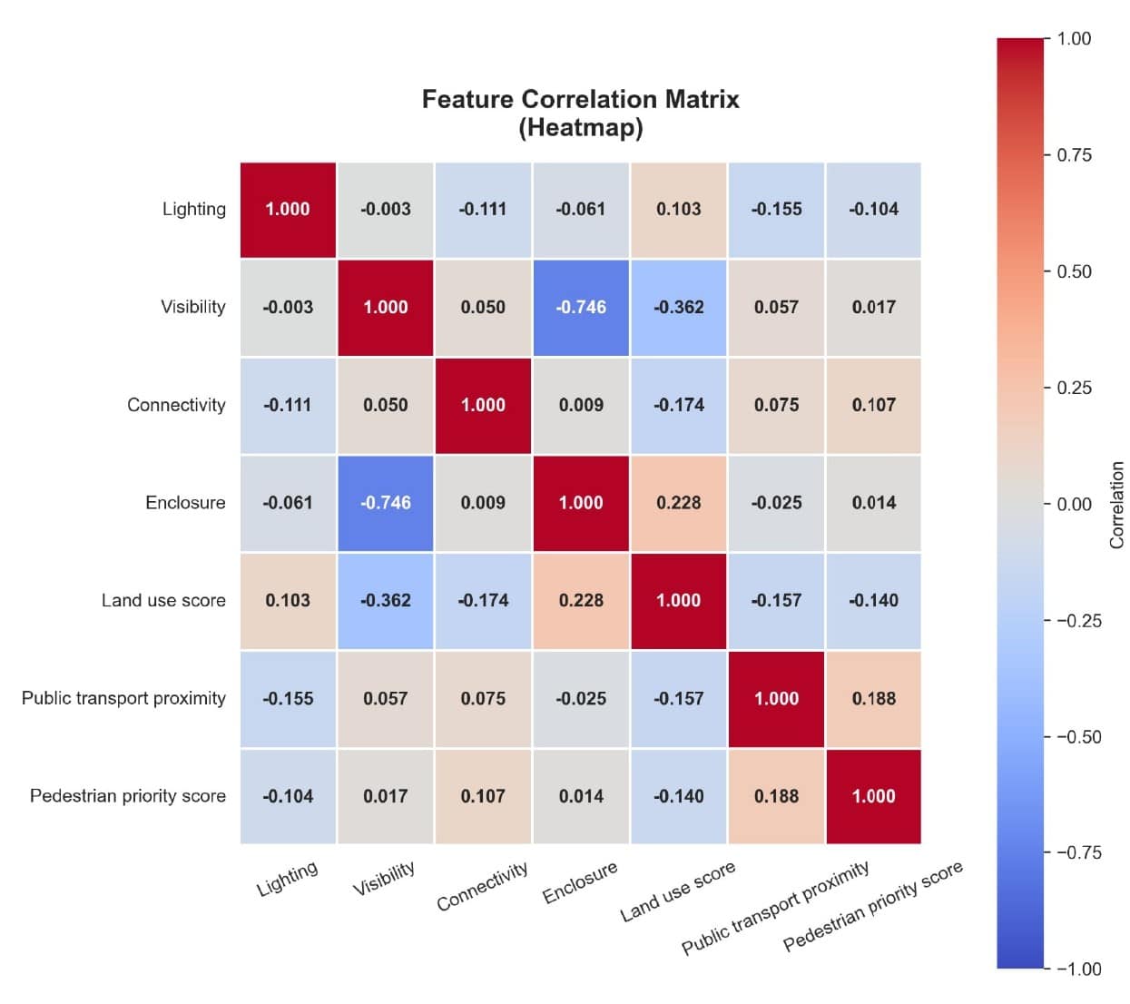
PCA: Redundancy check
PCA is our redundancy check. Most correlations are low — the one strong one is visibility and enclosure at -0.75: more enclosed streets are less visible. Nothing’s correlated enough to drop. Visibility dominates the first component, while lighting sits weak — consistent with the data sparsity we flagged. And to be clear: PCA is diagnostic; the clustering runs on the risk score.
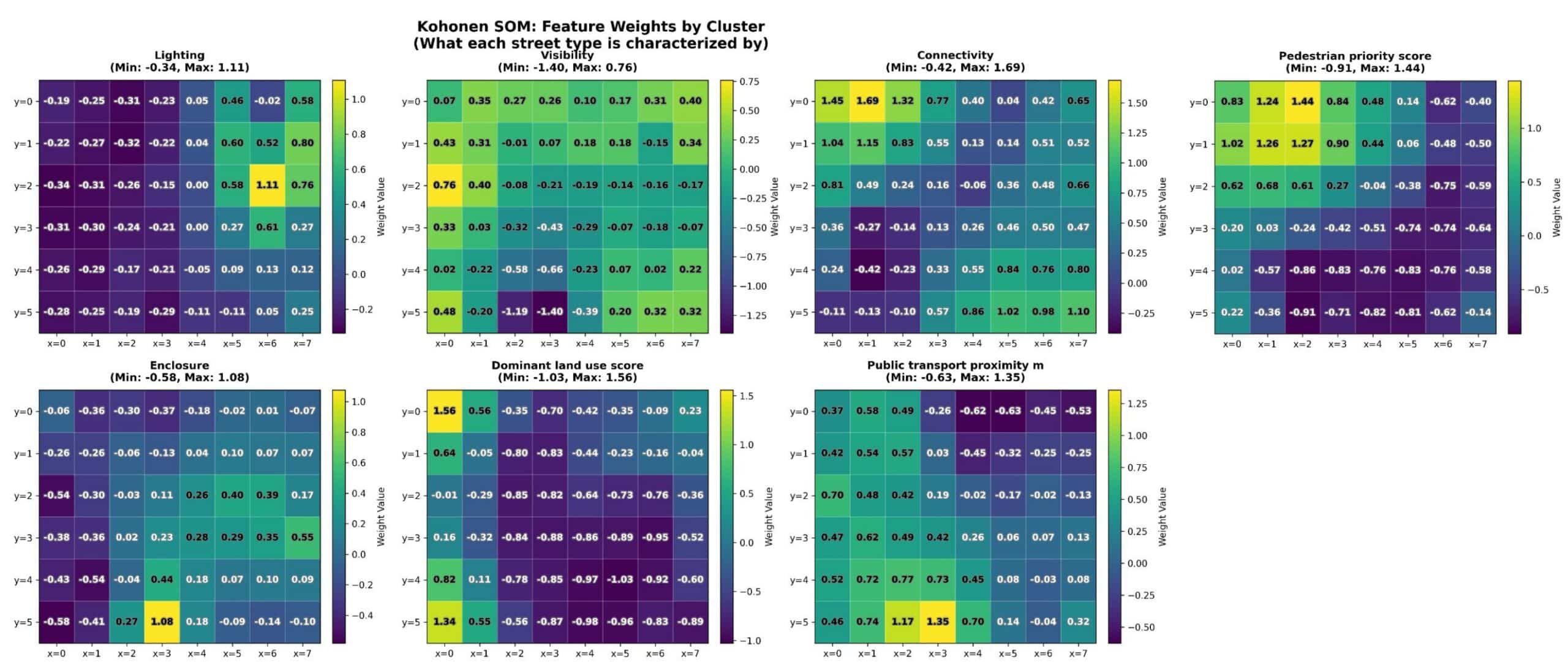
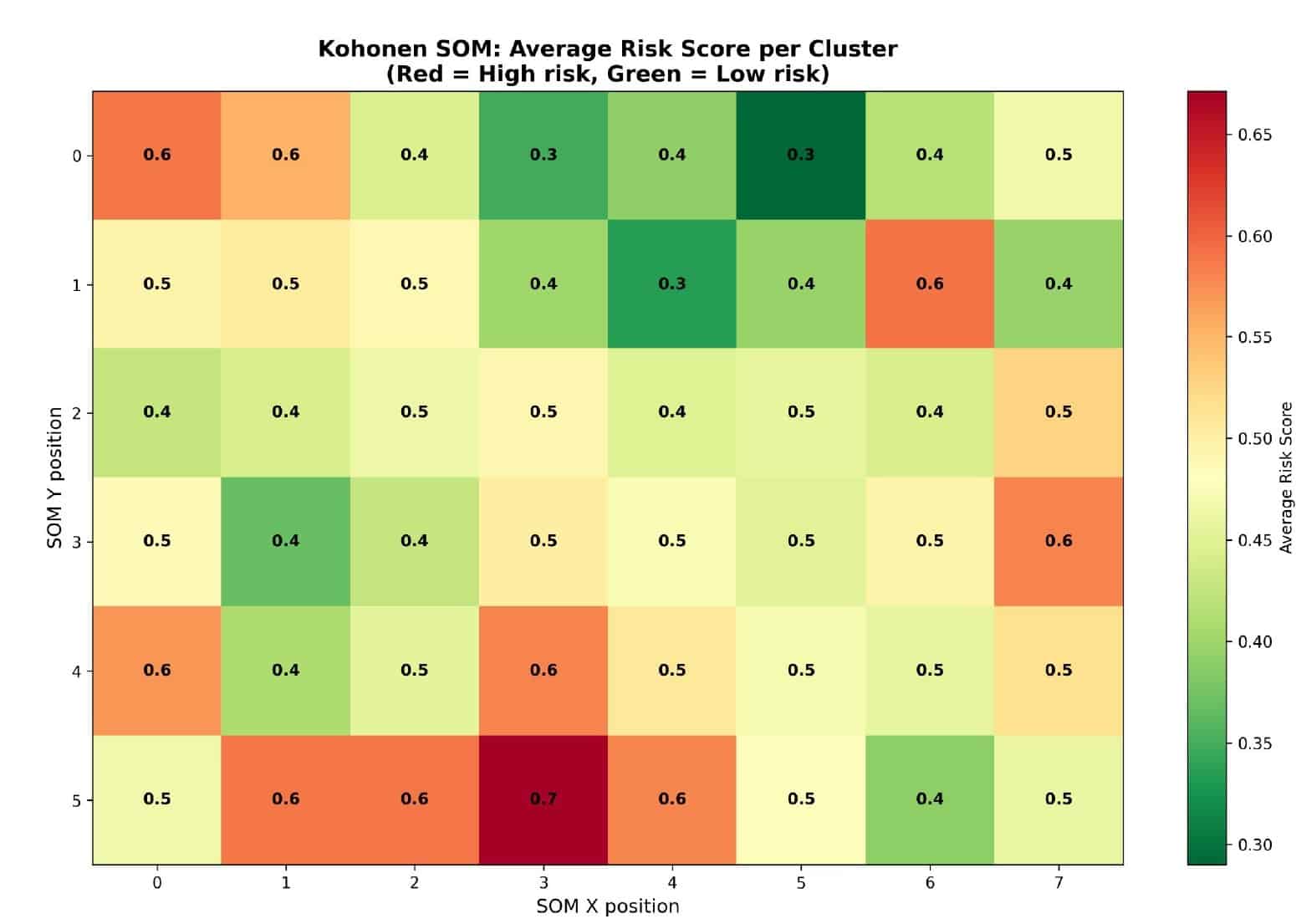
Kohonen map: coherent typologies, ambiguous risk
The Kohonen map sorts all seven features onto a 2D grid by similarity. The network organises into legible street types. But coloured by risk, near-identical cells show quite different values. Typologies describe street character; they don’t cleanly determine risk.
K-Means: Finding the natural breakpoints
K-Means cuts the score into three ordered classes. We chose k=3 — silhouette slightly favours two, but two only gives safe-versus-unsafe, and the ambiguous middle is where design intervention matters most. The split: 31% low, 47% medium, 22% high.
04. Model & Results
99% Accuracy – why that’s expected
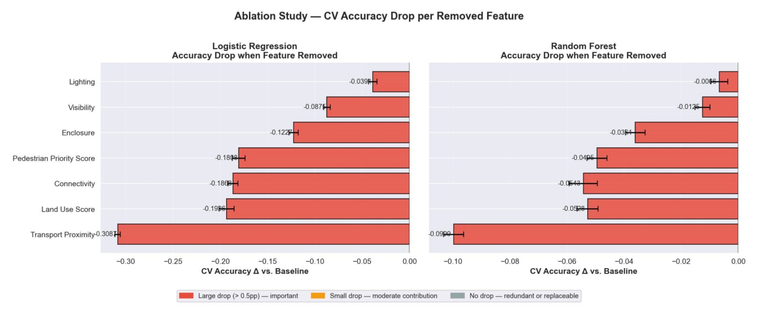
We tested Logistic Regression and Random Forest on 36,000 labelled segments. Logistic Regression hits 99% accuracy; Random Forest 95%. These numbers are expected by construction: the label was built from the same features the classifiers train on. Accuracy tells us the decision rule is clean and learnable — not that it’s correct. Logistic Regression beating Random Forest is also expected: our decision boundary is a linear threshold on a weighted sum.
The ablation study is more informative than the accuracy numbers. Transport proximity is the most important feature. Connectivity and land use follow. Pedestrian priority sits in the middle. Lighting contributes almost nothing to Random Forest — around 0.04 points. Lighting carries significant weight in the risk formula, yet near-zero impact when removed. The reason: Mapillary lighting is inconsistently mapped, many segments have no data. A feature that doesn’t vary cannot discriminate between classes. Feature importance = weight × variation. Zero variation, zero contribution.
Deployment
The deployment is an interactive visualisation built on the trained model. On any OSM street network: fetch features, run classification, render colour-coded segments. A proof of concept demonstrating the pipeline runs end-to-end on arbitrary OSM input.
05. Conclusions & Cross-City Deployment
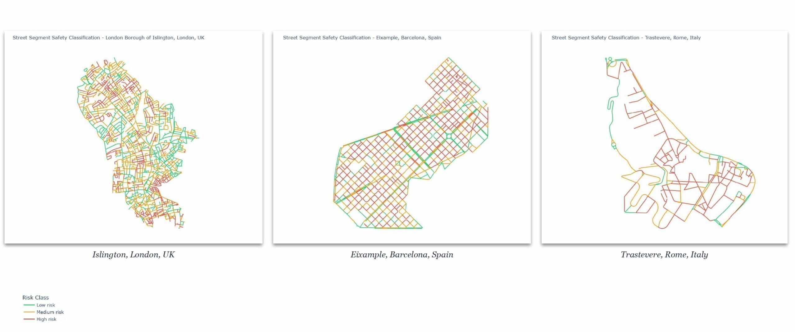
London trained, world tested
With London as training set, we applied the model to Barcelona’s Eixample and Trastevere in Rome. London’s Islington shows a mixed distribution. Eixample comes out almost entirely high risk. It is not a dangerous neighbourhood — but its orthogonal grid, high enclosure, and high connectivity map onto London’s high-risk feature region. The model isn’t wrong about what it sees. It’s wrong about what that means elsewhere.
SHAP: pinpointing the divergence
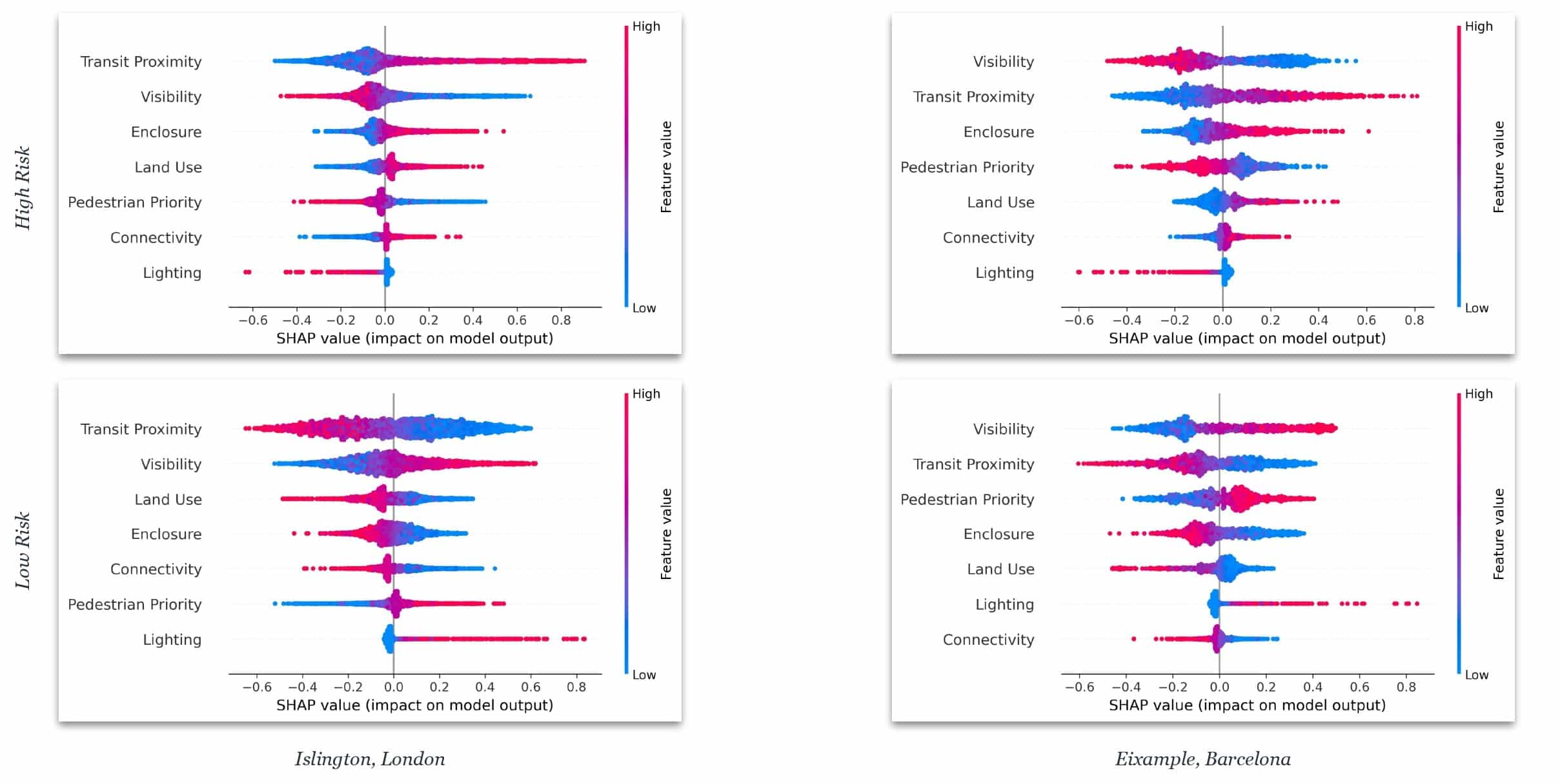
In London, high-risk predictions are driven by below-average connectivity and visibility — within the training distribution. In the Eixample, land use hits 3.35, visibility 2.35 — values the model has never seen. It extrapolates into high-risk by default. Not an architecture problem, not a feature selection problem: a per-city normalisation and distribution shift problem.
"K-Means centroids trained on London's morphology encode London's typology. They cannot be directly extrapolated to other urban contexts without re-fitting to those cities' own spatial baselines."
English cities: morphological kinship
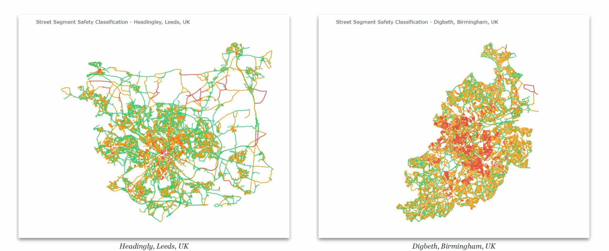
Applied to Leeds and Birmingham, distributions are more balanced. English cities share morphological history with London — similar fabric, network irregularity, building typologies. The model transfers better within a morphological family.
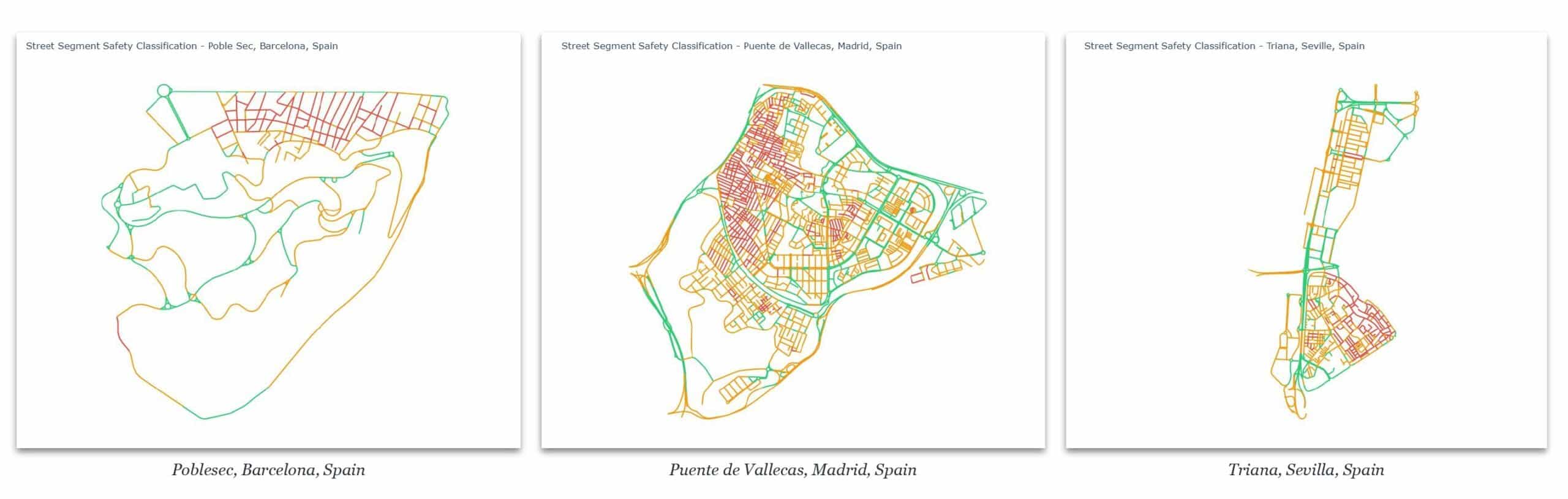
Training a second model: Barcelona
We re-fitted on Barcelona. Same pipeline, different dataset. The London model on the Eixample gives 695 high-risk segments, heavily skewed red. The Barcelona model gives a much more balanced result — dominated by orange, with green on the wider boulevards and red concentrated in the denser interior blocks. More balanced is not more correct — we still have no external ground truth. But across Spanish cities, the distributions are contextually plausible.
06. Conclusions
What we built — and what we didn’t
We built a pipeline that classifies street morphology, not street safety. Related, but not the same. Honest limitations: lighting data is unreliable; weights are expert priors, not learned from data; there is no external ground truth anywhere in the pipeline.
What we learned: spatial features can organise street segments into coherent, interpretable typological groups. The pipeline is portable within morphological bounds. The failures — normalisation, data quality, distribution shift — are precisely diagnosable. That diagnosability is itself a result.
"Street geometry is a meaningful input to safety classification — partially, under constrained conditions, within a single urban context, and only as a proxy for morphology rather than safety."
Open questions
Can sociological factors be encoded at all? Is the qualitative-quantitative gap bridgeable, or is it epistemological? Is human behaviour in space even predictable from physical environment? Being precise about where that uncertainty begins is the most honest contribution this project makes.
