Predicting Biking Station Vacancy in Barcelona

Introduction

Urban transportation planning relies on data science to explain the conditions driving mobility patterns. This exploration of bicing, Barcelona’s resident bike rental program, analyzes the actors impacting discrepancies in bicing data to select machine-learning strategies able to predict biking station vacancies across Barcelona for the year 2024 with an accuracy of 0.02387. With this understanding, tools can empower urban planners to optimize bicing allocation to adapt to shifts in demand.

Objective

Predicting the availability of vacancies at biking stations during a specific month of the year 2024 for the entire city of Barcelona.

Value of Preciding Bicing Vacancy

1. Optimization of Resources: Urban planners can better allocate resources, ensuring that bikes and docking stations are available where and when needed.
2. Enhanced User Experience: Users can rely on the availability of bikes and docks, improving the adoption of bike-sharing programs.
3. Informed Infrastructure Development: Data-driven insights can guide the development of new stations and the enhancement of existing ones, tailored to actual usage patterns.

Methodology

Our approach was structured in three main phases: Data Gathering, Data Cleaning, and Model Implementation:

1. Data Understanding
   • Before gathering new data, our team investigated the bicing test dataset which consisted of:
     • location data in the form of x, y coodinates and the identifier of the origin bicing station;
     • availability data containing bicing availability by type: mechanical, e-bike, and overall; and
     • temporal data, breaking down availability by the year, month, day, and hour.
     • Additionally, a dataset on the bicing stations was analyzed for its geographic attributes, mostly altitude.
   • This initial understanding of data guided our model development process.
2. Data Gathering:
   • To support our understanding of the spatial relationships that determine bicing availability, we generated bounding boxes of 1km2, buffers with radii of 500m, and isochrones of a five minute walk radius at a pace of 4.8 km/h using the networkx package within the walk network.
   • The generated isochrones provide an understanding of accessibility and were the elected geometry to qualify open data within relevant boundaries.
   • Within these geometries, we collected a variety of data from OpenStreetMaps (OSM) using the osmnx package, including amenities (ie: restaurants, cafes), transportation alternatives (ie: public transport stations), and land use data (ie: residential, educational, commercial).
3. Data Cleaning:
   • We removed irrelevant columns, handled missing data, and corrected out-of-range dates.
   • Outliers were eliminated using the quantile method, ensuring our dataset was robust for modeling.
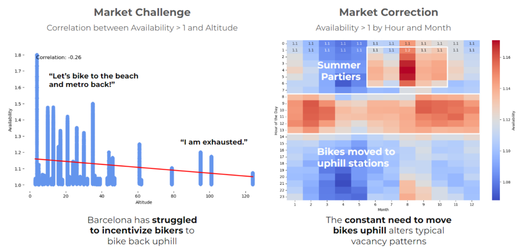
   • Key to the strategy was removing availability values outside the 0-1 range, as stations correlated with availability values over 1 related to the preference to ride downhill.
4. Model Implementation:
   • We explored various models, focusing on supervised learning models best able to synthesize categorical data.
   • After a thorough evaluation, we focused on ensemble learning methods like Random Forest and CatBoost for their robustness and efficiency in handling complex datasets.

Data cleaning and preparation

Trends and Correlations

Our analysis is based on the following hypothesis:

• Understanding existing data

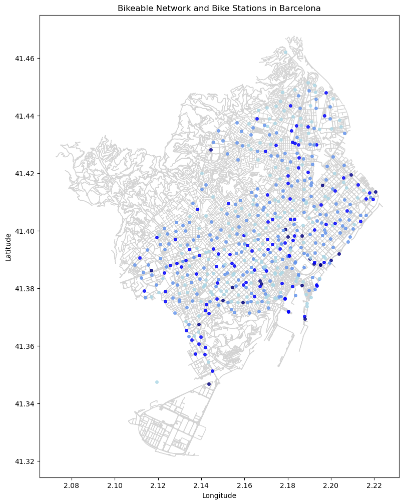
To understand the existing data, it is necessary to plot bike availability and location on a map to perceive the data in a spatial context. From this visualization, we can observe that bike station frequency is higher in the city center and urban areas compared to peripheral regions. Additionally, bike availability tends to be lower near the beach due to higher demand in these areas.

To understand the existing data, it is necessary to plot bike availability and location on a map to perceive the data in a spatial context. From this visualization, we can observe that bike station frequency is higher in city centers and urban areas compared to peripheral regions. Additionally, bike availability tends to be lower near the beach due to higher demand in these areas.

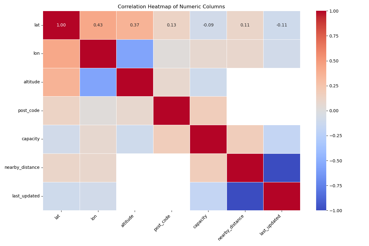
In terms of data correlation, we recognize that temporal factors such as day, month, or year have less correlation with bike availability. This can be attributed to noise or outlier data, such as the impact of COVID-19 in 2019 or special events, which can mislead the model’s accuracy. By understanding these influences, we can compare model predictions by either adding more datasets and factors or removing certain temporal data to determine which approach improves model accuracy.

New dataset

• Topography challenges: The natural inclination to avoid uphill biking led to lower usage of certain stations.
  • This challenge of geography led to bikers taking bikes in the morning from high altitude locations to low altitude locations. As a result, locations near the beach were prone to high availability after the morning commute and those near the mountains were susceptible to a gap in supply by 2pm.
  • The city recognized this challenge in 2021 and corrected for it by moving bicycles uphill between 11am and 2pm.

/

• Inverted Infrastructure: Areas with dense alternative transportation options showed different usage patterns, necessitating a balance between bike and other transport modes.

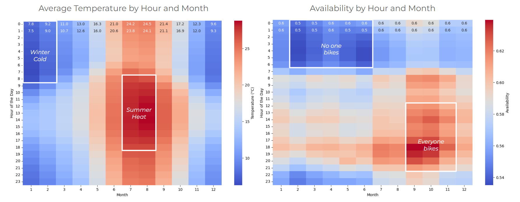
• Seasonal Patterns: Availability varied significantly with seasons, influenced by factors like weather and tourism.

Key Takeaways

• Data Relevance: Excluding altitude, bike network, or supply, and alternative infrastructure, or demand data would cloud rather than support predictions as the city self-corrects for demand influenced by geography, bicing infrastructure is inversely correlated with transit infrastructure, and the transit alternatives are bear no correlation to availability.
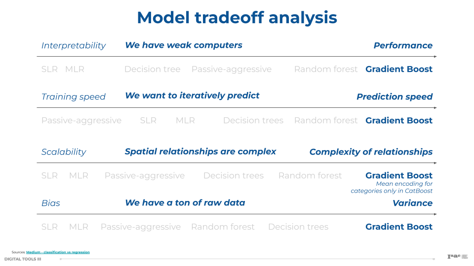
• Model Selection: Choosing the right model is the most crucial step when using machine learning. CatBoost and Random Forests were particularly effective due to their handling of categorical data and prevention of overfitting.
• Data Utilization: Combining multiple years of data does not always mean a better model accuracy, but rather higher noise and slower codes.

Model implementation

Models Explored

Our team focused on the use of supervised learning models. These models learn from labeled training data to make predictions. Our data was powerful, with over 186,000 rows over five study years.

1. Passive-Aggressive Regressor: The Passive-Aggressive Regressor is an online learning algorithm that adjusts the model as new data comes in.
   • Pros:
     • Efficiency: Suitable for large datasets and real-time applications due to its online learning capability.
     • Adaptability: Quickly adapts to changes in data distribution, making it useful for dynamic environments.
   • Cons:
     • Stability: Can be sensitive to outliers and noisy data.
     • Complexity: Requires careful tuning of hyperparameters to achieve optimal performance.
2. Multiple Linear Regression (MLR): MLR models the relationship between two or more features and a continuous target variable by fitting a linear equation to observed data.
   • Pros:
     • Simplicity: Easy to implement and interpret.
     • Efficiency: Requires minimal computational resources, making it fast to train.
   • Cons:
     • Linearity Assumption: Assumes a linear relationship between features and the target, which may not capture complex patterns.
     • Sensitivity: Can be affected by multicollinearity among features and outliers.
3. SGD Regressor: The Stochastic Gradient Descent (SGD) Regressor is an iterative method for optimizing an objective function with suitable smoothness properties.
   • Pros:
     • Scalability: Efficient for large-scale datasets due to its iterative nature.
     • Flexibility: Can be used with different loss functions and regularizers.
   • Cons:
     • Convergence: Can be slow to converge, especially with noisy data.
     • Hyperparameter Tuning: Requires careful tuning of the learning rate and other parameters.
4. Random Forest: Random Forest is an ensemble learning method that constructs multiple decision trees and merges them to get a more accurate and stable prediction.
   • Pros:
     • Robustness: Reduces overfitting by averaging multiple trees, providing stable and accurate predictions.
     • Feature Importance: Offers insights into feature importance, aiding in feature selection and understanding.
   • Cons:
     • Computationally Intensive: Requires significant computational resources for training and prediction.
     • Complexity: Less interpretable compared to simpler models like linear regression.
5. CatBoost: CatBoost is a gradient-boosting algorithm that handles categorical features efficiently and prevents overfitting.
   • Pros:
     • Performance: Excellent accuracy, especially with categorical data.
     • Ease of Use: Handles categorical features natively, reducing the need for preprocessing.
   • Cons:
     • Training Time: Can be slower to train compared to simpler models.
     • Resource Intensive: Requires substantial computational resources.
6. LightGBM: LightGBM is another gradient-boosting framework that uses tree-based learning algorithms, optimized for speed and efficiency.
   • Pros:
     • Speed: Faster training speed and lower memory usage compared to other gradient-boosting algorithms.
     • Scalability: Capable of handling large datasets with higher efficiency.
   • Cons:
     • Complexity: Can be complex to tune and may require substantial effort to achieve optimal performance.
     • Interpretability: Less interpretable compared to simpler models.

Prediction

Model Performance

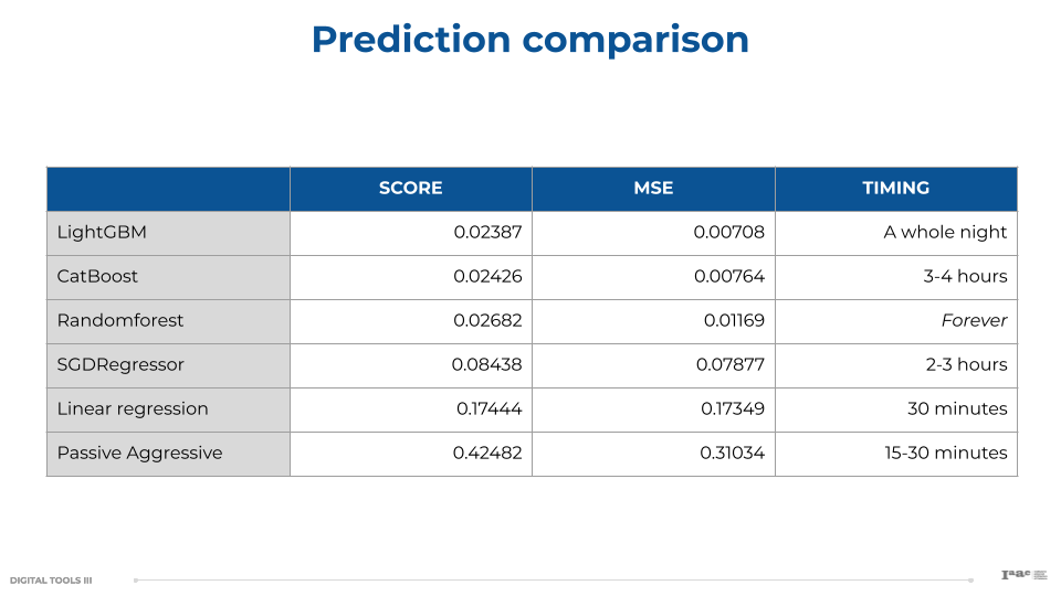
In order to evaluate the performance of each model and compare their results, we used an MSE analysis. Mean Squared Error (MSE) is a widely used metric to measure the performance of a regression model. It represents the average of the squared differences between the actual and predicted values.

MSE provides a quantitative measure of how well a model’s predictions match the actual data. Here’s why it’s important:

1. Accuracy Assessment: MSE helps determine how close the predictions are to the actual values. A lower MSE indicates better performance.
2. Error Sensitivity: By squaring the differences, MSE penalizes larger errors more than smaller ones. This sensitivity to outliers can help in improving model accuracy by focusing on reducing large deviations.

A low MSE Indicates that the model’s predictions are very close to the actual values, signifying high accuracy; meanwhile a high MSE suggests that the model’s predictions deviate significantly from the actual values, indicating poor performance.

Another critical factor alongside prediction accuracy was the ability to handle large datasets efficiently. Our dataset comprised millions of records, which posed significant challenges in terms of data processing, model training, and resource management. With millions of data points, our computers sometimes ran out of memory. Efficient memory management was crucial to ensure that the data processing and model training could be completed without crashing the system.

Model Selection

Given the constraints of handling large datasets and the need for efficient training times, we had to balance between model accuracy and computational feasibility. Our choices were influenced by:

• Resource Availability: Limited computational power and memory forced us to prefer models that were not only accurate but also efficient in terms of resource usage.
• Model Efficiency: Models like LightGBM and CatBoost struck a good balance by providing high accuracy with reasonable training times, making them suitable for our large dataset.
• Scalability: Methods that could scale well with increasing data size without a proportional increase in memory and time requirements were preferred.

Based on these factors, LightGBM and CatBoost emerged as the top performers in terms of prediction accuracy. LightGBM slightly outperformed CatBoost but took longer to train. Random Forest, while robust, was impractical due to its extensive training time. Simpler models like Linear Regression and Passive-Aggressive Regressor, though quicker to train, did not provide sufficient accuracy for our needs.

This evaluation highlights the importance of balancing accuracy and computational efficiency when selecting models for practical applications.

Next Steps

With more time to improve the model, we may take the following next steps:

• Iterative runs: To analyze and understand the source of the variance in the model, we may systematize the analysis of variance with scenarios of variable weighing.
• Feature engineering: By experimenting with feature consolidation, we may improve the speed of the model. Transforming existing features may uncover hidden patterns in the data and improve predictive power.
• Cross-validation: To generalize the model and improve its ability to handle outlier or unrecorded times, we may run the model on many subsets, varying the percentage of test data in the test-train split.
• Add new data: While we were unable to locate any external data helpful to increasing predictive power, we have hypothesis about additional data that would have been helpful to improving the model.
  • New construction: Data on year-over-year additions of bicing stations and replacement of bikes may account for variance between years.
  • Behavioral patterns: Public event data, made available by the Adjuntament de Barcelona, may account for variance in availability at specific nodes and hours.