Beginnings
Our project’s concept is to develop a classification model that identifies street intersections (graph nodes) in Stockholm, Sweden, susceptible to flooding during a 100-year flood event. Based on our initial research, we found that graph machine learning operates at three levels: the graph, its edges, and its nodes. With access to a 100-year flood simulation for the entire city, we initially aimed to train our model to classify streets (graph edges) with flood risk. However, given the studio’s pace and scope, we narrowed our focus to node classification. We experimented with removing the flooding data and adjusting the model’s learning rate.
In this project, we comprehensively analyse urban road networks utilizing geographic and data science techniques. The project integrates geospatial libraries such as Geopandas, NetworkX, and OSMnx to import, manipulate, and visualize geographic data. Our primary dataset is sourced from OpenStreetMaps in XML format, containing intricate details of city road networks. We pre-process the data to project it into the appropriate coordinate reference system (CRS) and handle any missing values. Subsequently, we focus on analyzing the permeability of nodes and edges within the network, which involves calculating node valences and assigning permeability values based on specific urban planning metrics. The analysis culminates in visualising the road network with permeability values, utilizing colour mapping techniques to depict variations effectively.
Additionally, the project delves into the application of machine learning for classification tasks within the context of road networks. Using PyTorch and DGL, we construct and train a graph neural network model to predict the classifications of different nodes. We evaluate the model’s performance by comparing ground truth labels against predicted labels, utilizing confusion matrices and visualization techniques to illustrate the results. The workflow includes saving and loading the trained model for reproducibility. Through this project, we aim to provide valuable insights into urban road network characteristics and demonstrate the utility of advanced data science and machine learning methods in geographic analyses.
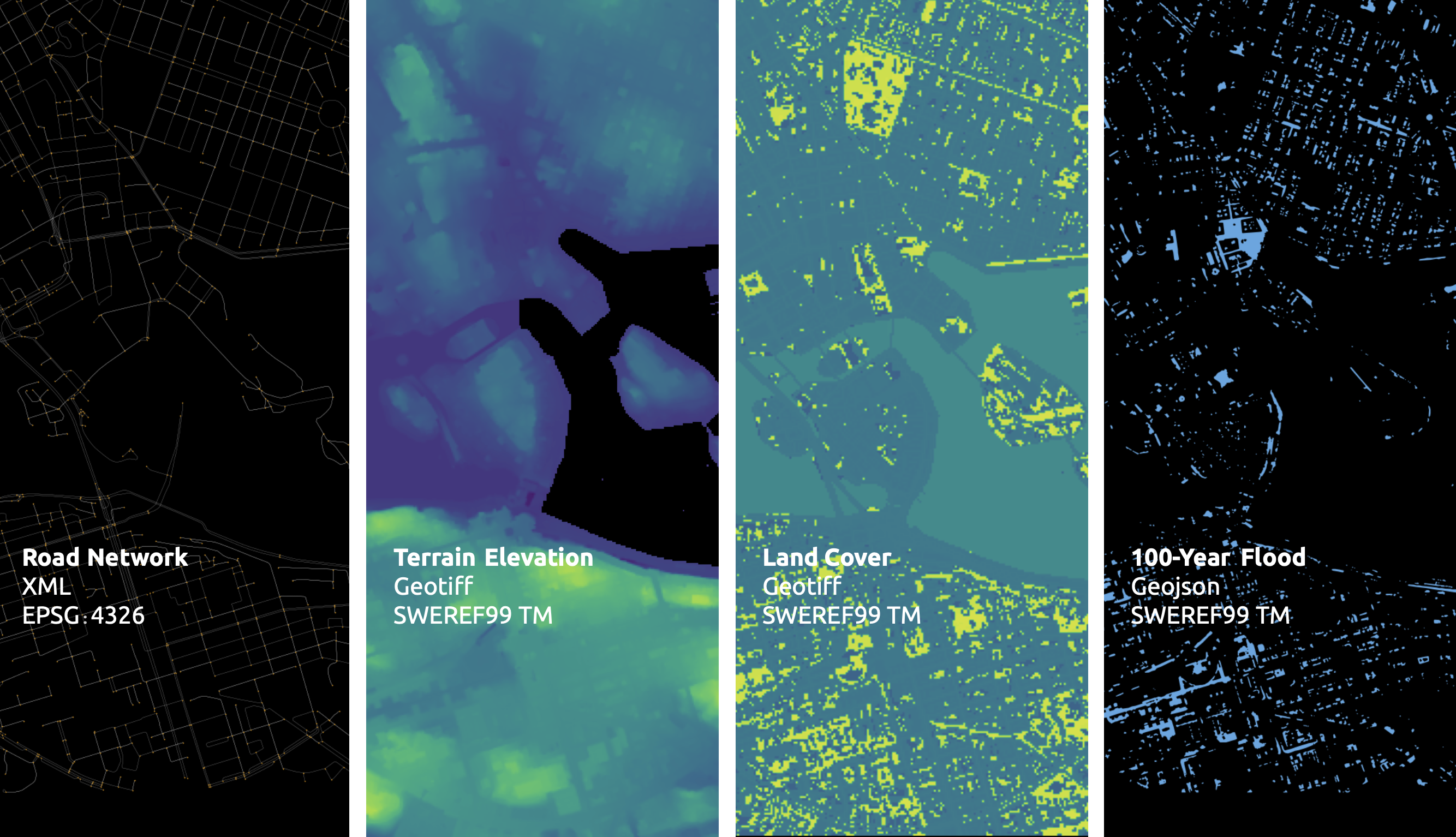
Our first challenge was harmonizing different file formats and projections. For operations requiring data from both, we temporarily reprojected our road network to match our .geotiff files. The Python libraries Rasterio and GDAL were essential for data extraction.
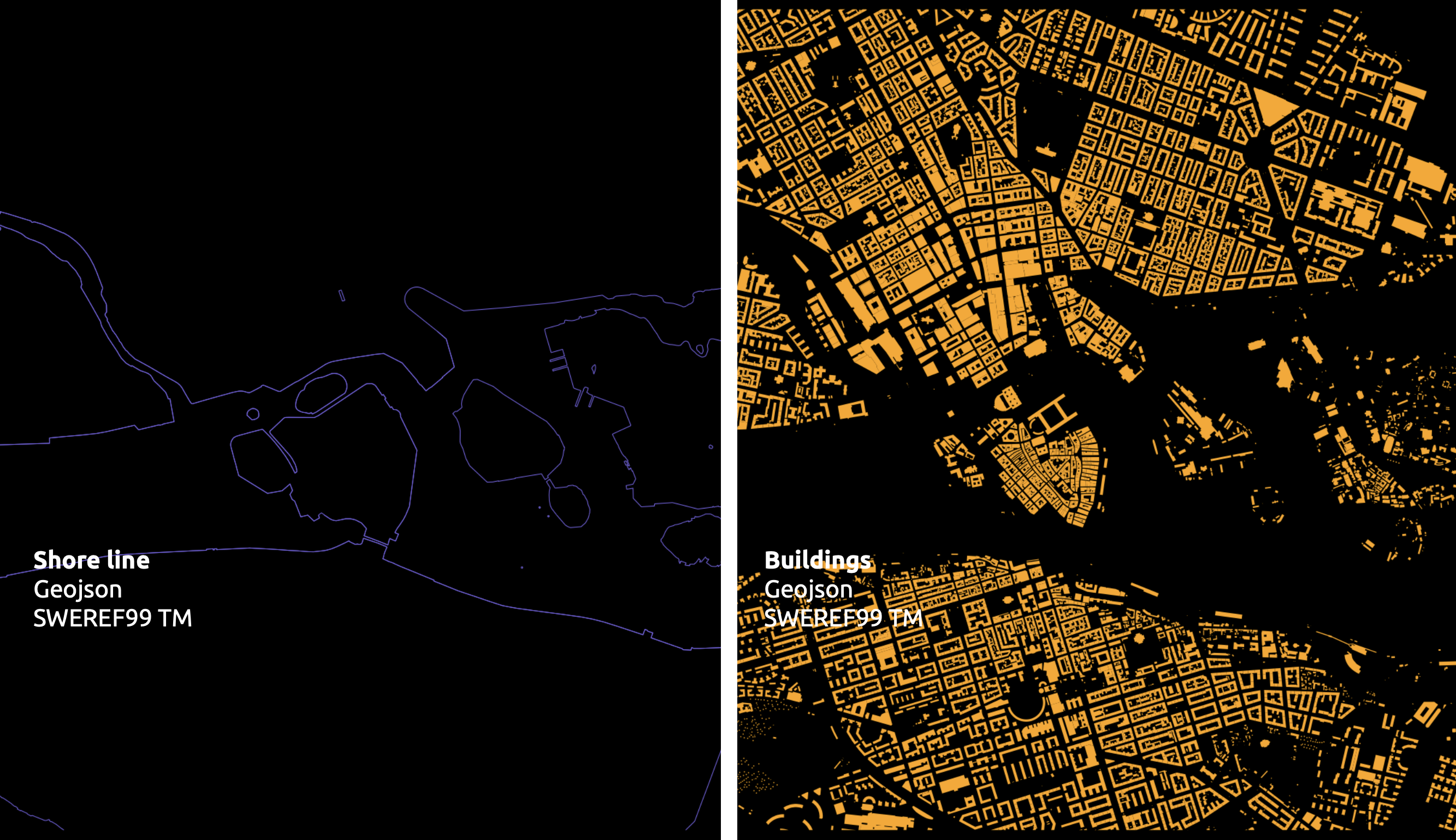
Given Stockholm’s archipelago, visualizing the road network was challenging. So, we incorporated shoreline and building datasets to distinguish built areas from parks. We focused on graphics from the start, learning to overlay mixed datasets for better visualization.
First Trials
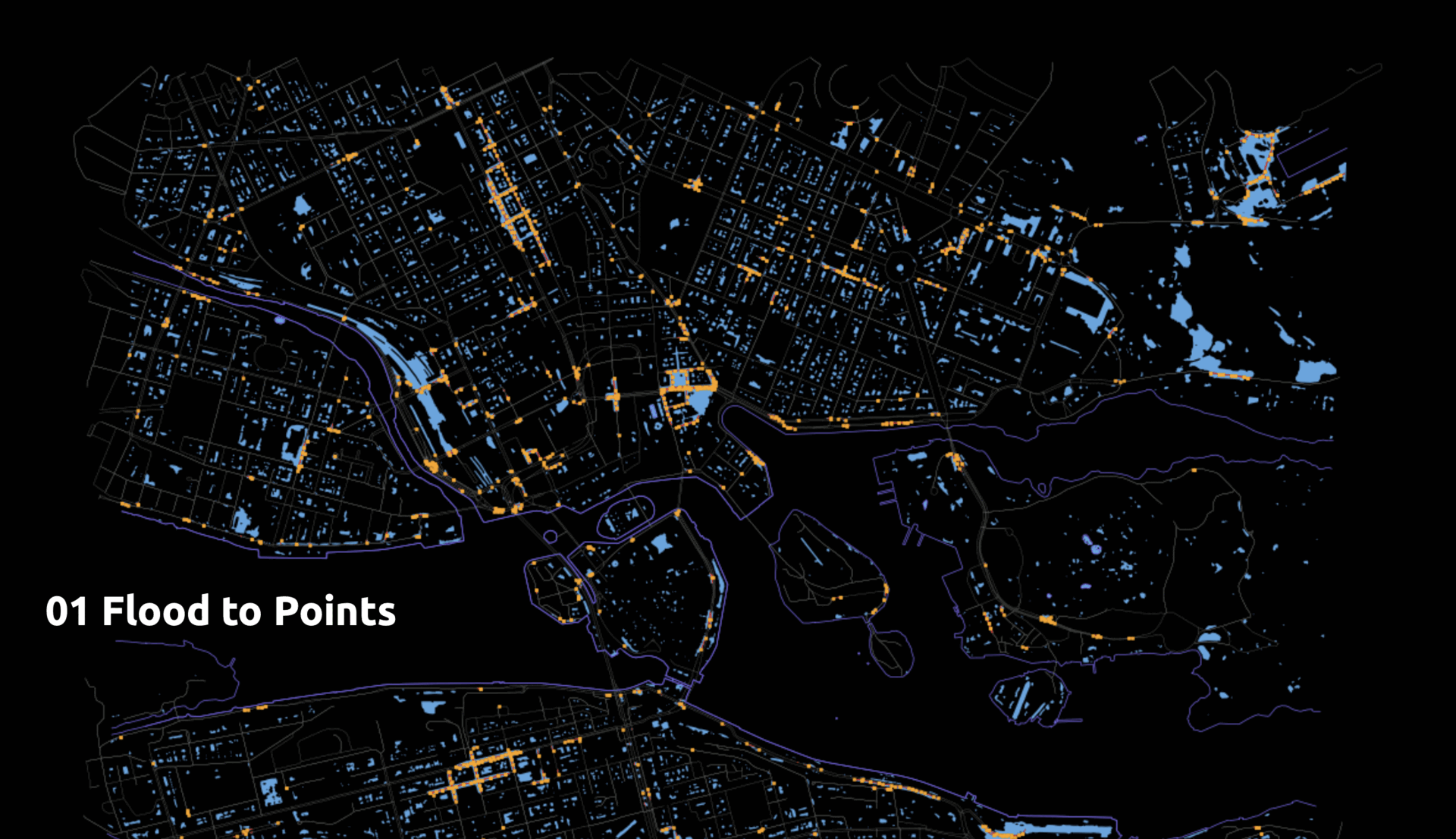
Here a quick sample of the embedding and encoding we produced initally. Among those:
- Flood value to point along streets (edges)
- Nearest Edges to Flooded Points
- Flooded Streets and Key Infrastructure
- Topographical Elevation to nodes
- Slope between two nodes as edge feature
Second Trials
In this second round of trials, we tested adding features to edges. This time we tried:
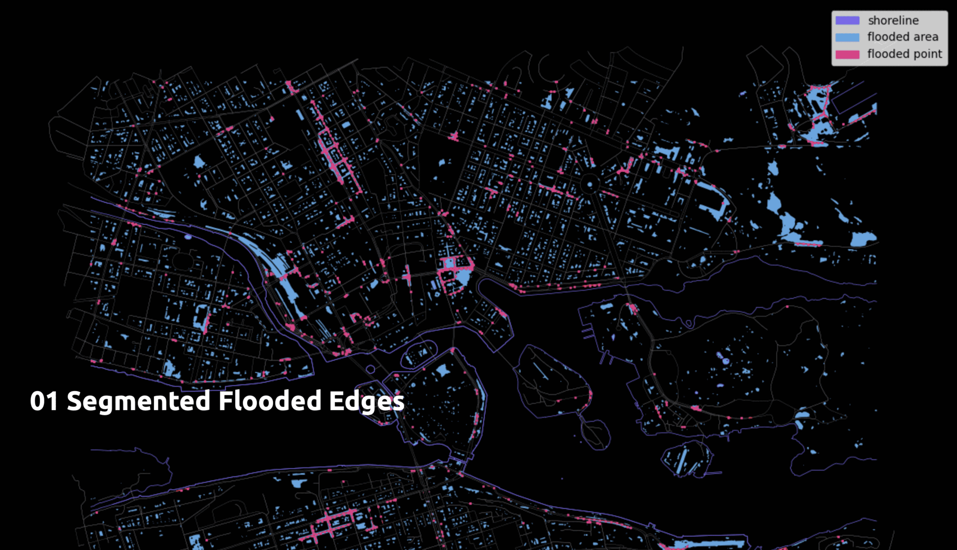
- Segmented flooded edges
- Edge flood risk
- Land cover to nodes
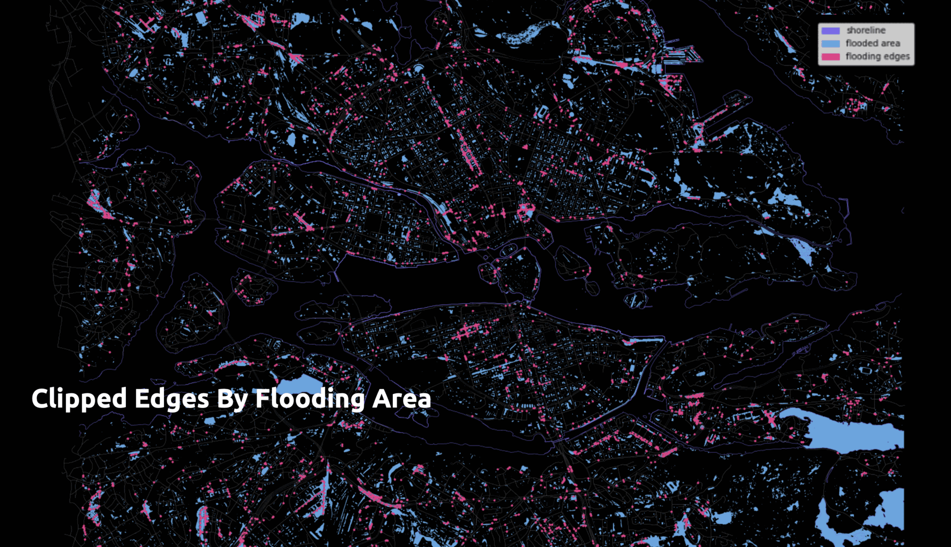
Some edges were longer than the flooded areas. To address this, we segmented the edges so smaller segments could fall entirely within a flood area and be considered flooded.
Based on elevation and the previous segmentation, edges were classified as fully flooded or at risk of flooding.
Nodes acquire the land cover type directly beneath them.
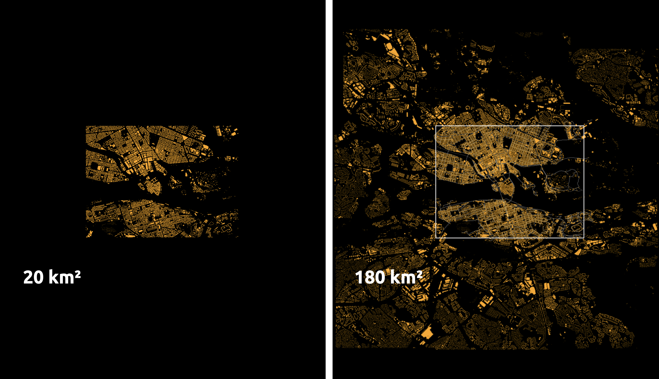
Initially, we used a dataset covering 20 km² but realized the model needed more data. We increased the dataset size ninefold, which improved the model’s performance and taught us how to stitch together .geotiff and .geojson files.
Data Encoding
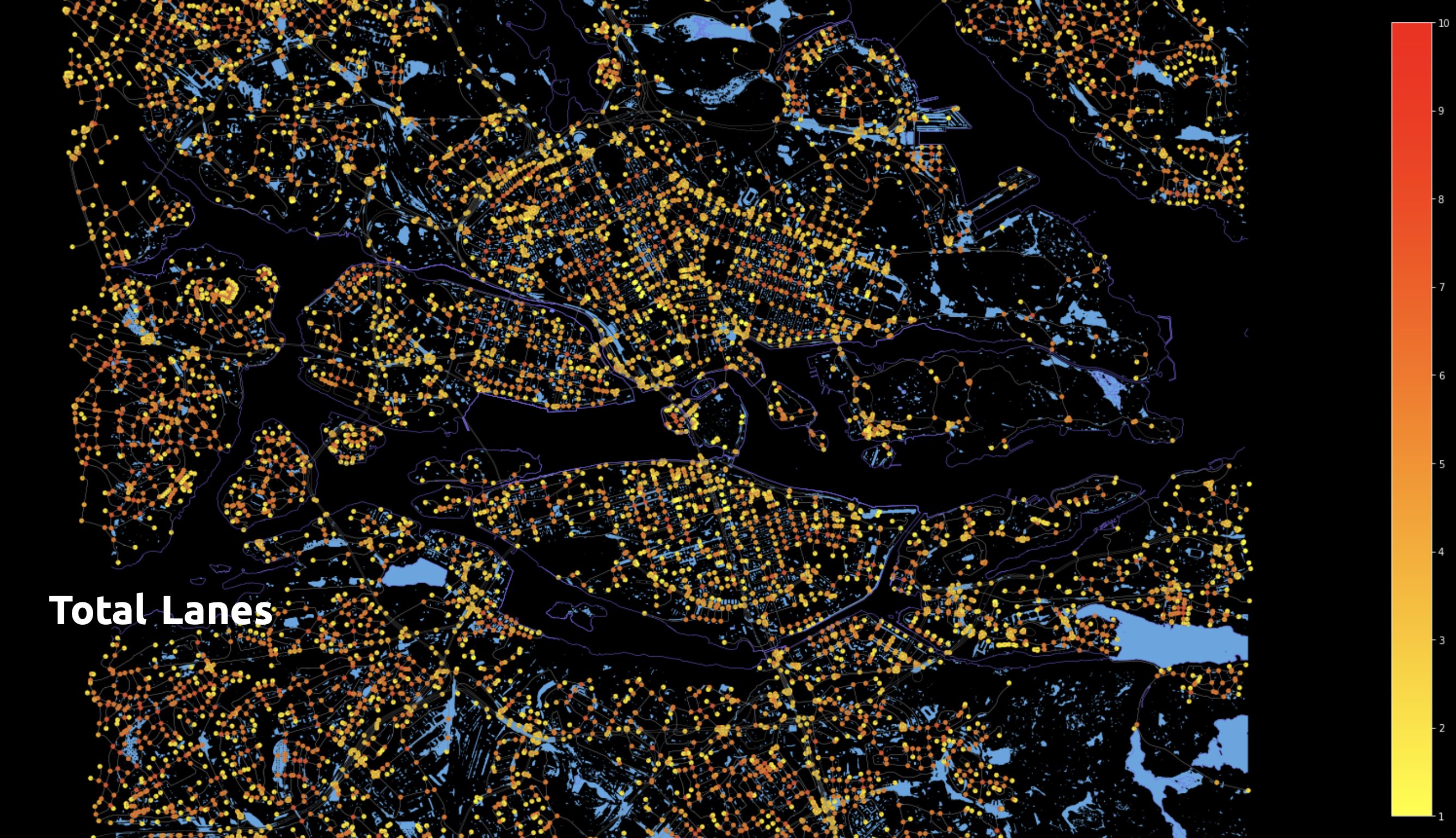
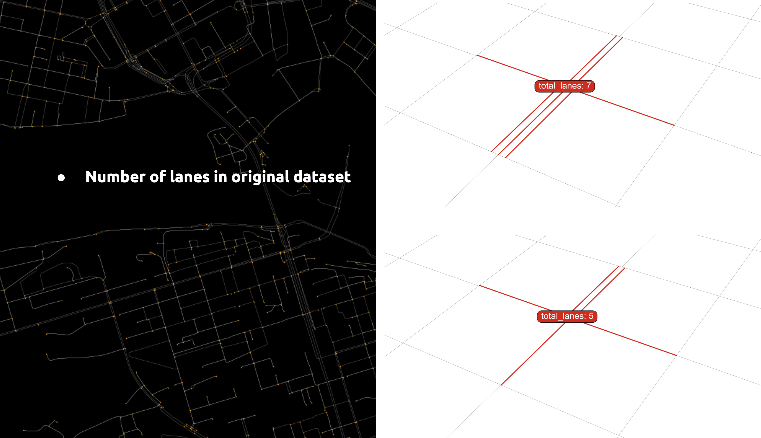
Feature 01 – Total Lanes
We found the ‘lanes’ in the connected edges for each node, accumulated the number, and assigned it to the node.
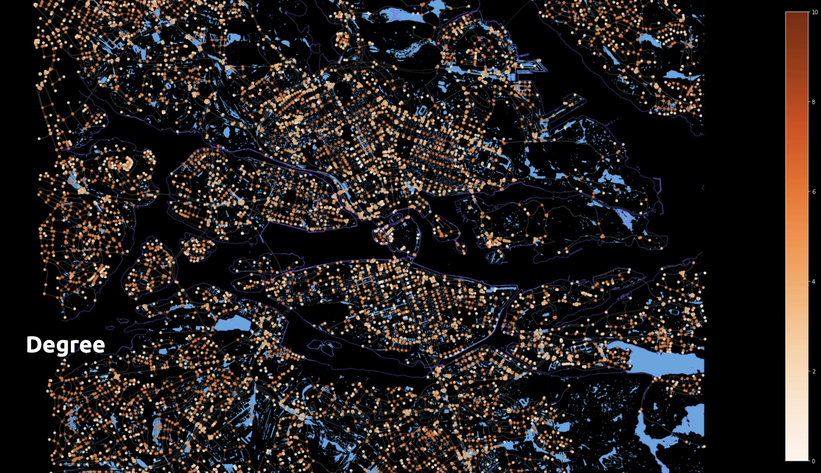
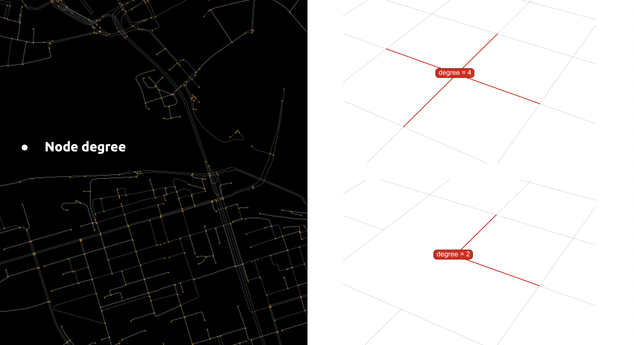
Feature 02 – Degree
We used the node’s degree to determine how many streets converge at a single point, making it one of our node features.
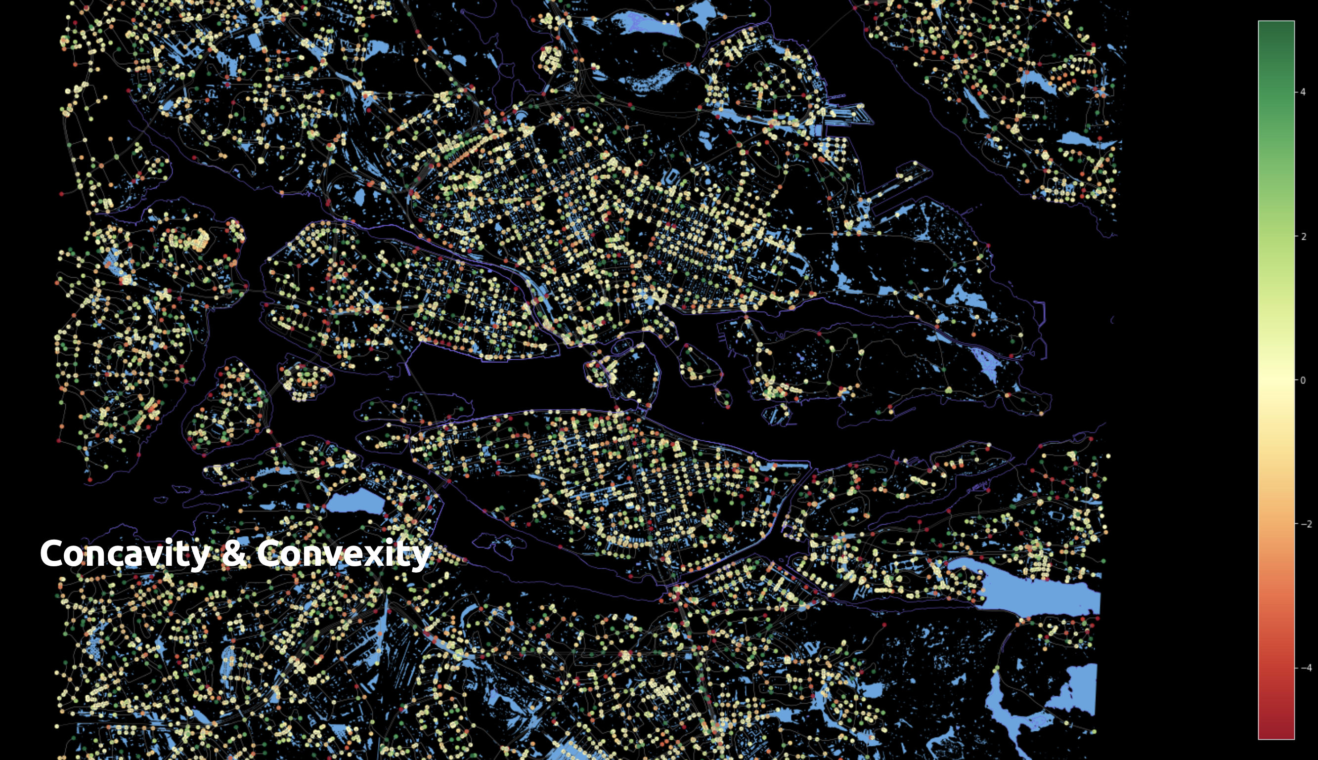
Feature 03 – Concavity & Convexity
To relate node elevation to flooding, we calculated the mean elevation of each node’s neighbours and subtracted it from the node’s elevation. This way, we encoded the elevation of the area surrounding each node.
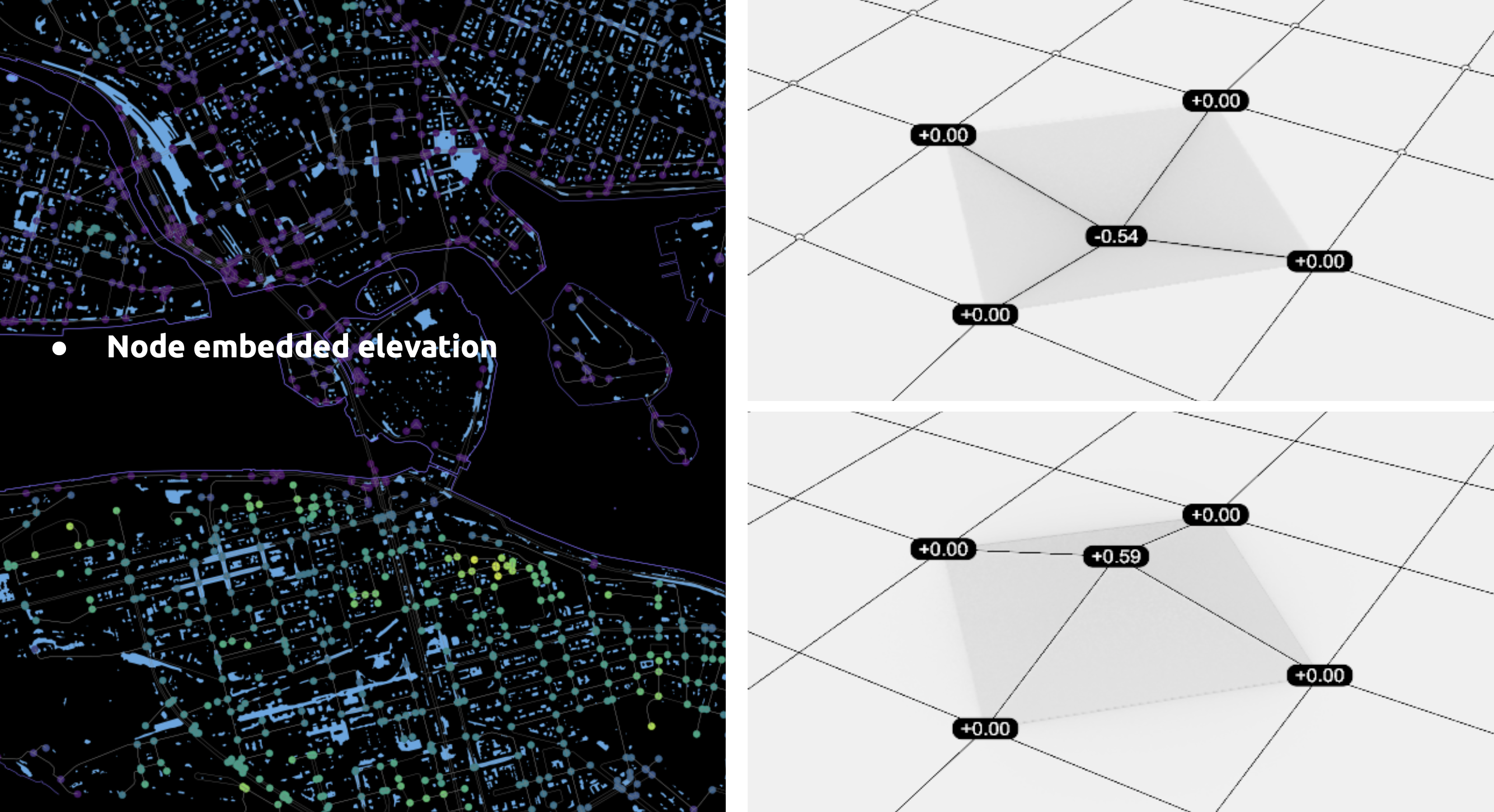
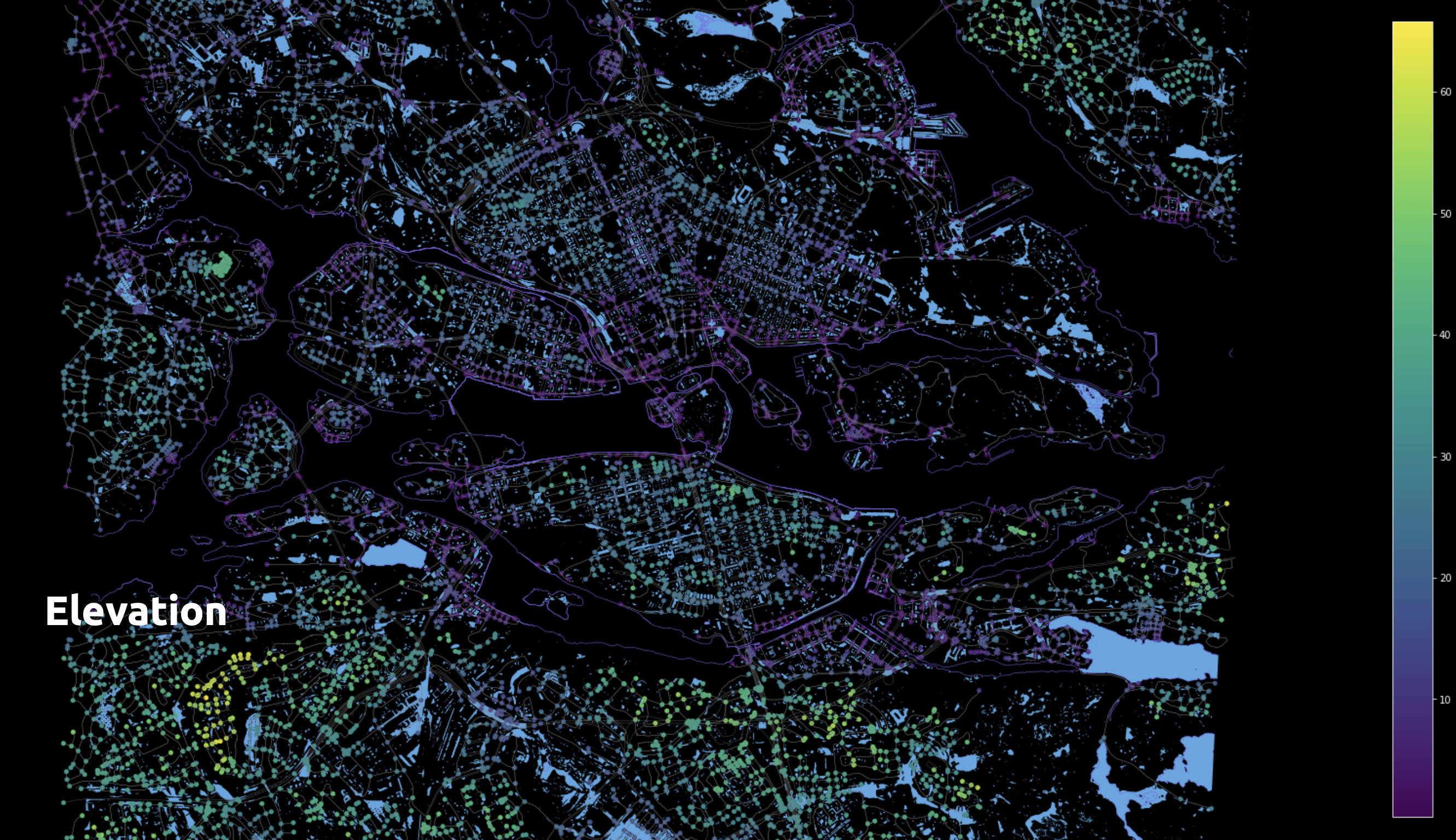
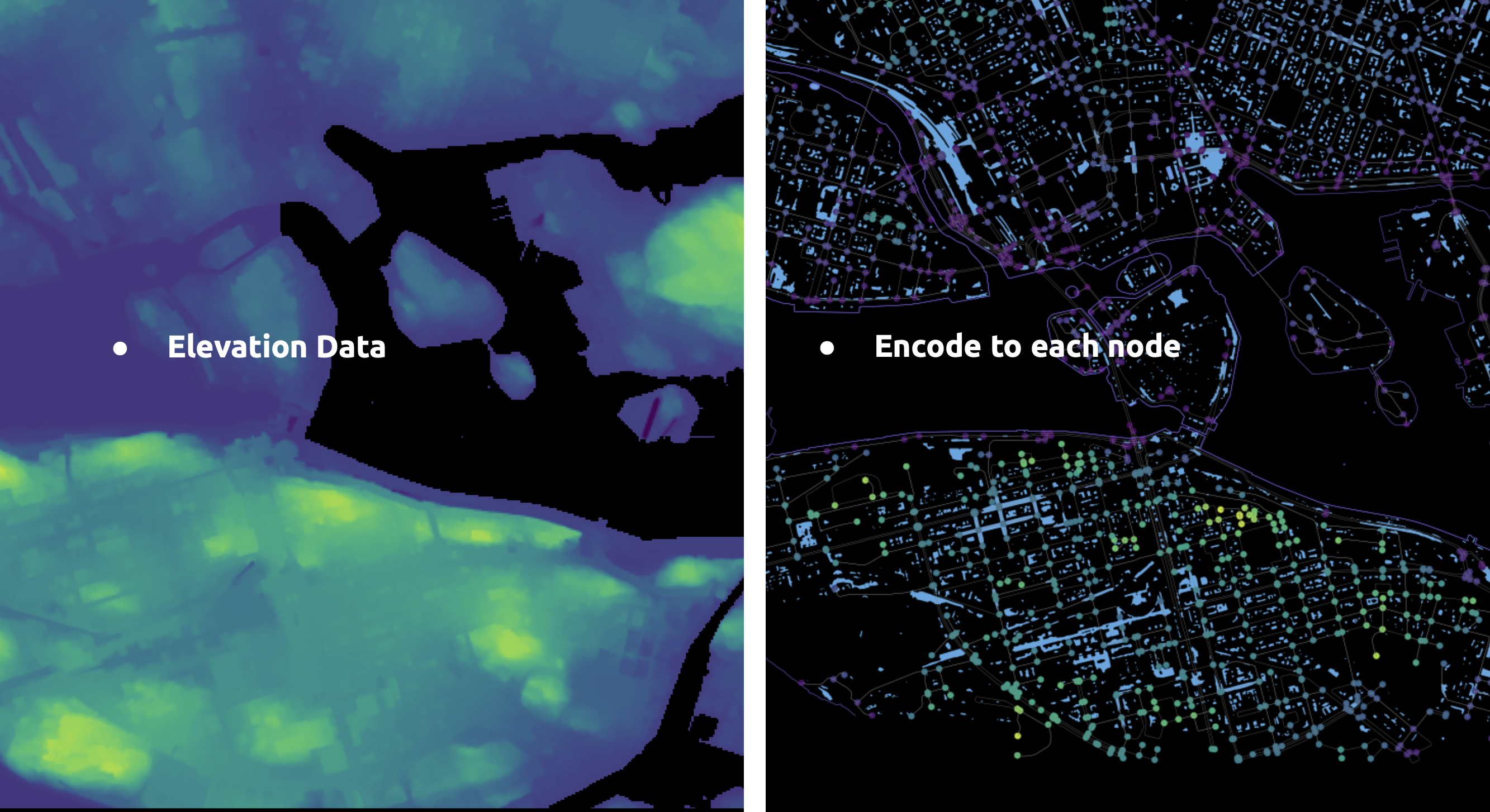
Feature 04 – Elevation
The OSMnx graph is overlaid with the .geotiff elevation file, and nodes acquire the elevation directly beneath them. The Rasterio and GDAL libraries were key for this translation.
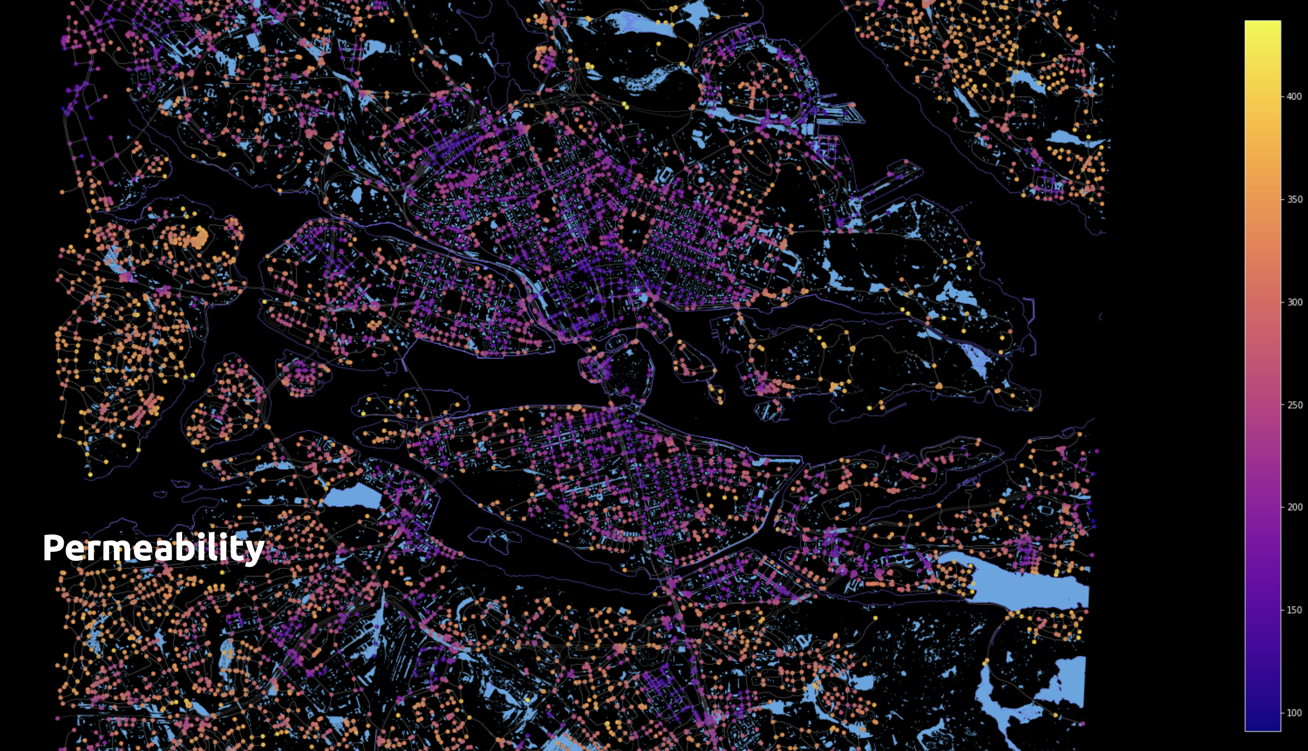
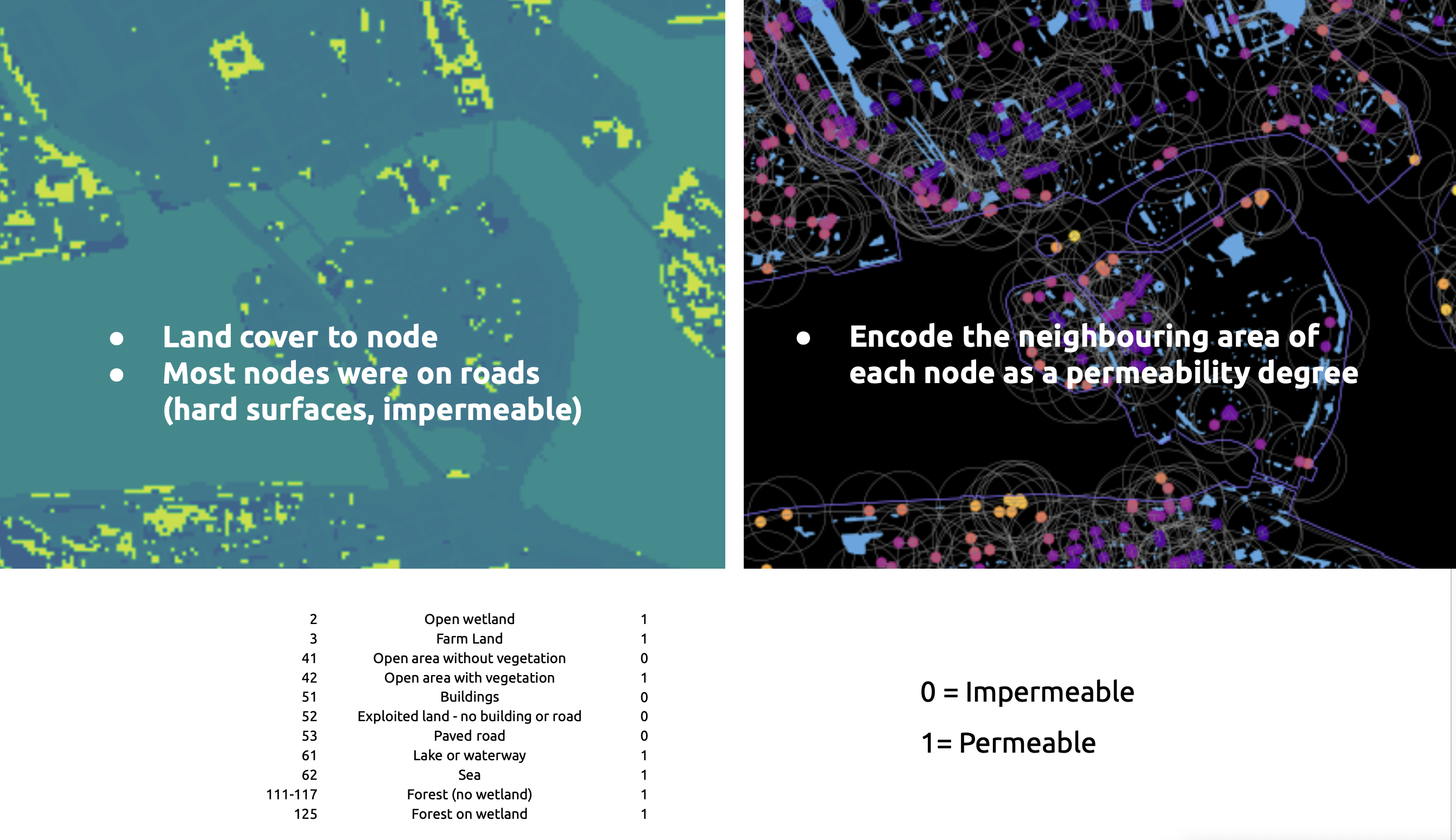
Feature 05 – Permeability
Initially, we mapped the land cover value right under the node, but since most nodes are on the streets, we missed other land cover types. So, we encoded the neighbouring area within a 100-meter radius around each node. Pixels within circles of impermeable land covers, like buildings or paved roads, were assigned a value of 0. Pixels with permeable land covers, like farmland, forest, and wetlands, were assigned a value of 1. These values were summed and added to the node as a feature called permeability.
Labelling Nodes
Due to the large number of nodes, finding nodes in flooded areas was too slow. Instead, we identified edges in flooded areas, clipped them, and divided them to create temporary points. On these temporary points, we created bounding boxes. The graph’s nodes inside those boxes got labelled as flooded or not flooded.
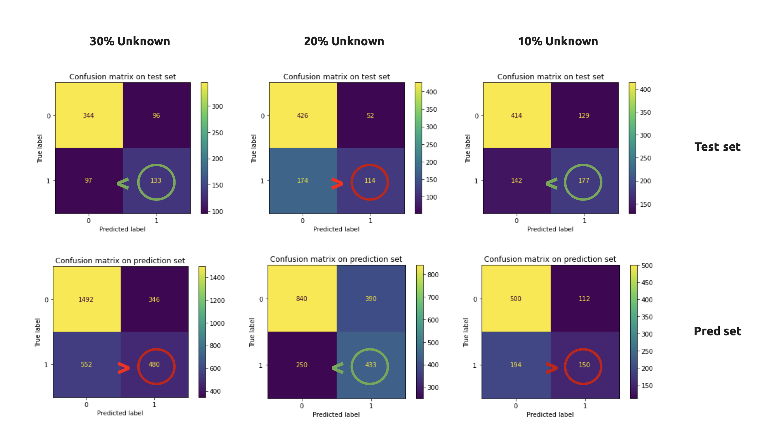
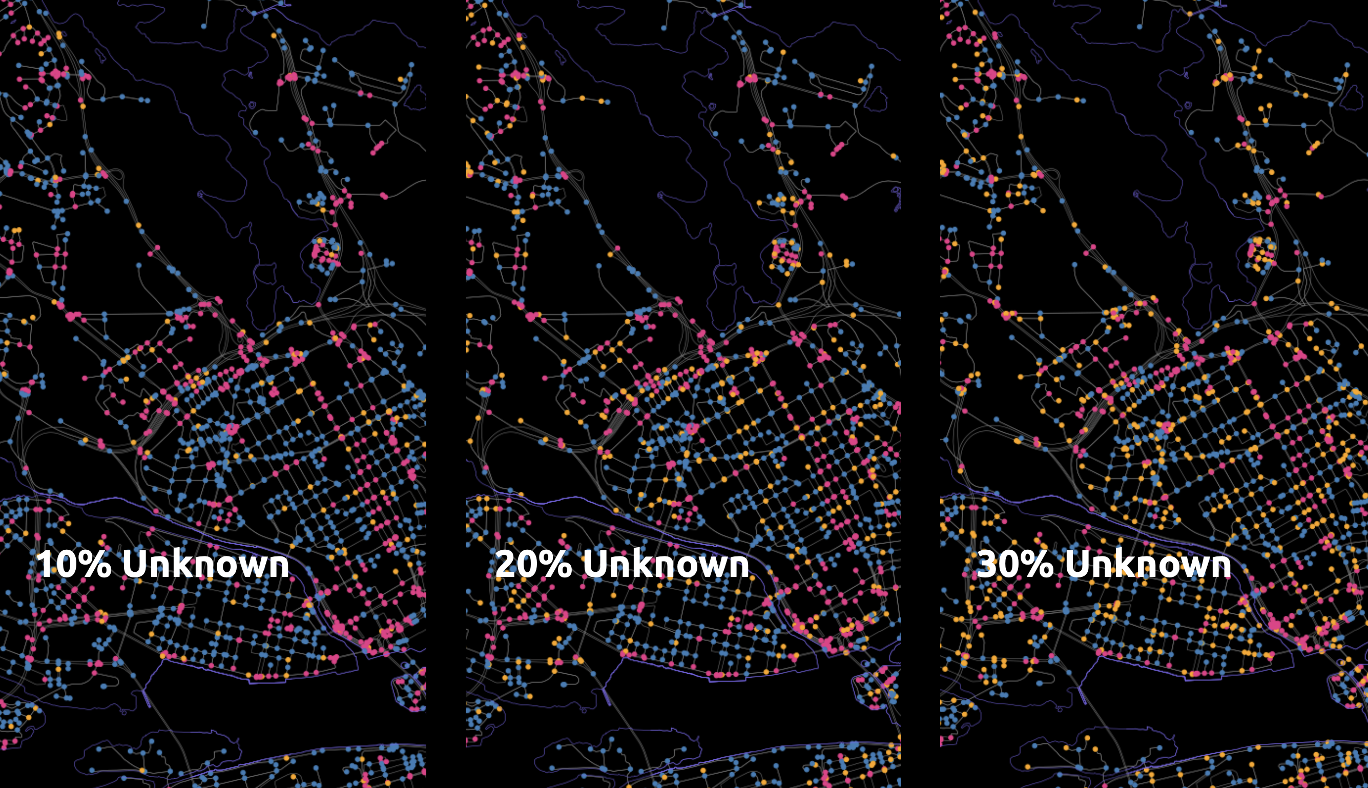
To test our model, we changed the classification of 20% of the nodes to an additional class 3, called “unknown”.
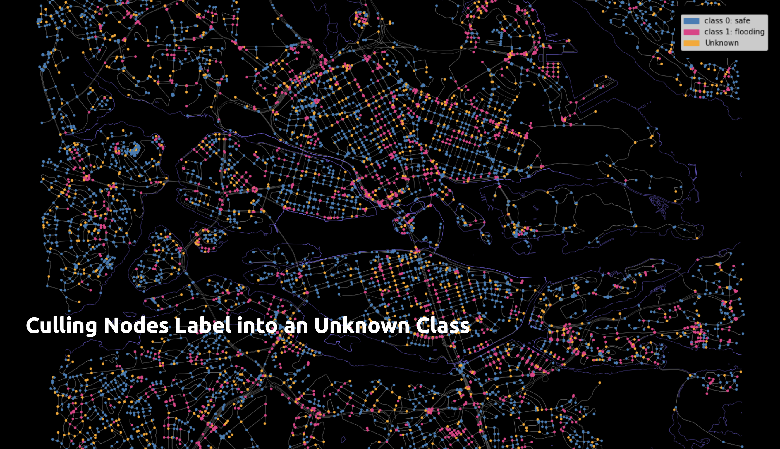
We experiment with various test cases that vary in the percentage of unknown nodes.
Model Training
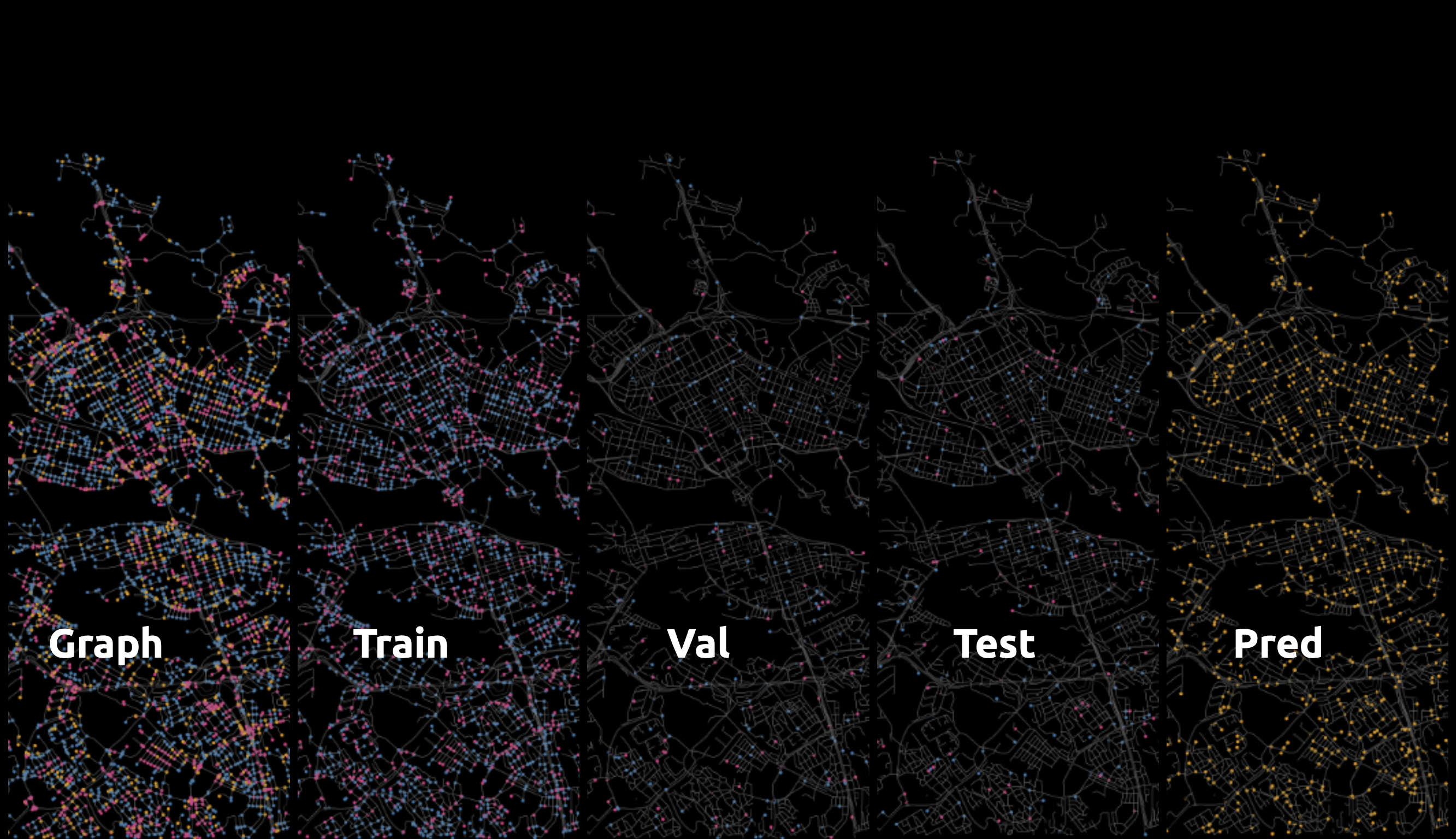
This is how the graph looks in different Dataset splits
The F1 score is what we use to assess how well the classification task was performed. A model performs better with fewer unknown nodes it contains. When we had more data, we discovered that. Better results and inverse relationships will be obtained with fewer hidden layers.
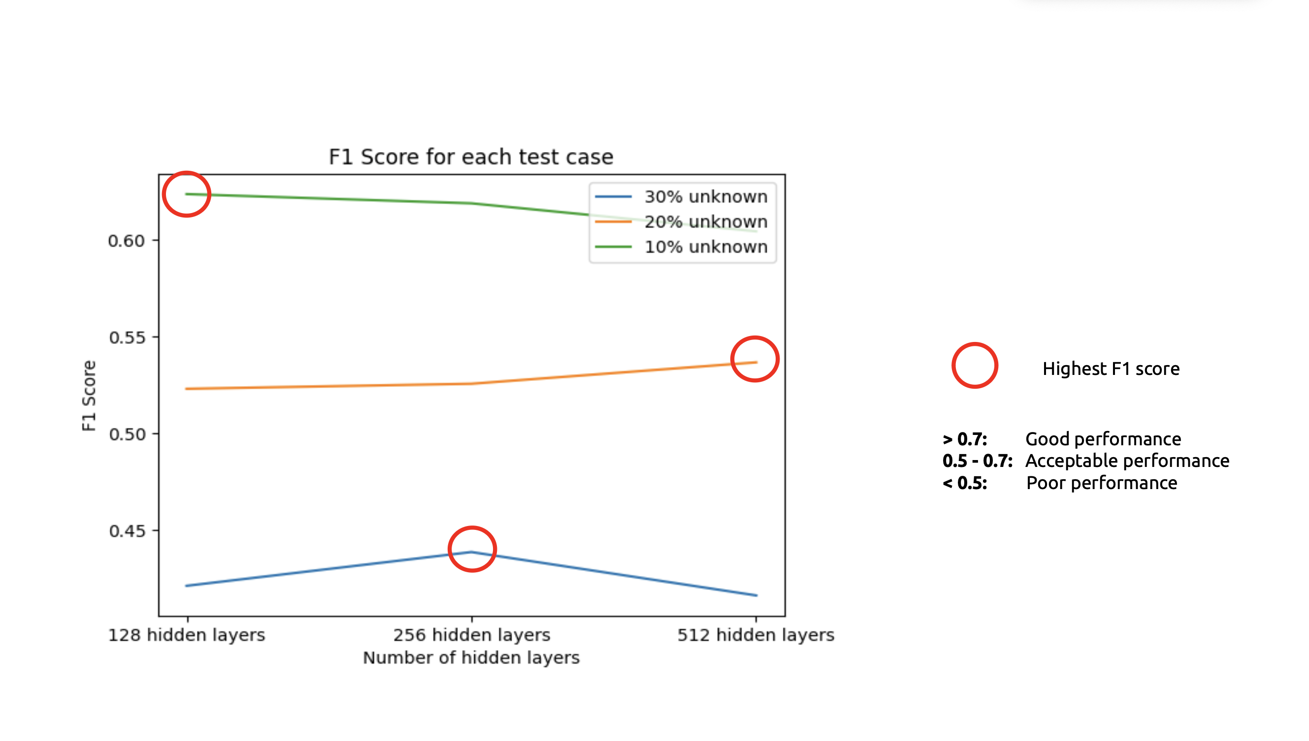
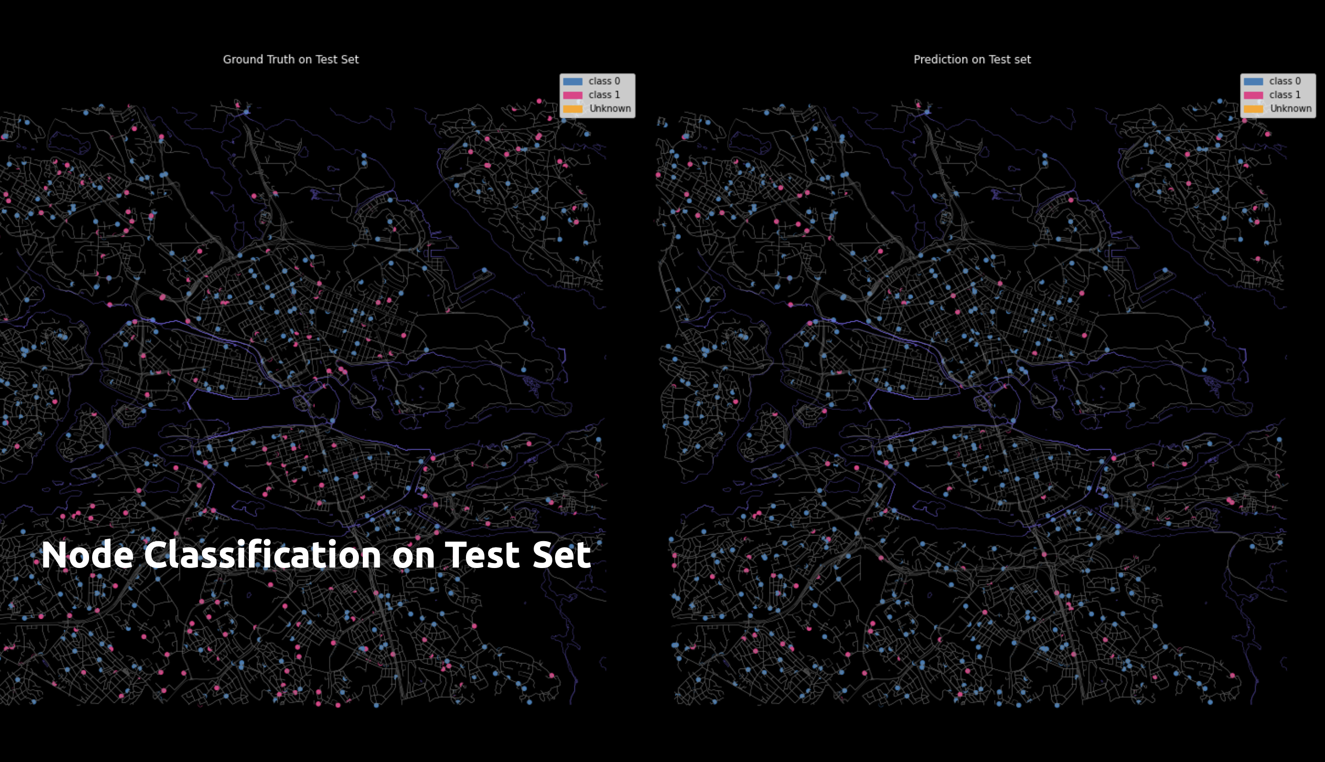
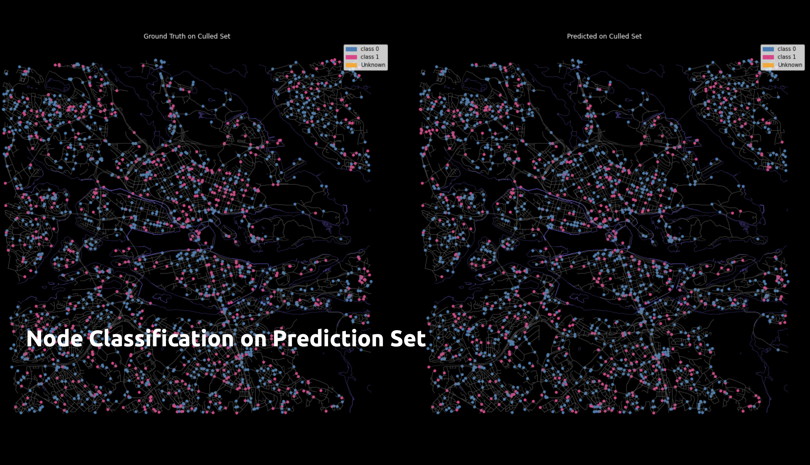
It’s interesting to note that, most of the time, the performance of the test set and prediction set is inverse. The prediction set will be poor if the test set performs better.
Although there isn’t a conclusion yet, our current features may be insufficient to determine the flood risk. Perhaps information regarding the sewer system or watersheds should also be provided as features.