
Abstract
3D-SOLIDS Component Classification tool utilizes machine learning to optimize the placement of essential 3D components such as walls, doors, windows, floors, and railings in residential floor plans. By analyzing spatial features and architectural attributes, it automates and enhances the design process, ensuring accuracy, consistency, and compliance with building standards. This tool aids architects and designers by reducing manual effort, improving design efficiency, and facilitating better collaboration and communication, ultimately leading to more sustainable and customized architectural solutions.
Team: BAO Q. Trinh, Manolya Nielsen, Hetal Bharwani, Agustin Salas

We are explaining the structure and the workflow for processing 3D unit models in our machine learning project.
Dataset
- Components Table: The table on the left lists various components of the unit models, including their IDs, types (e.g., Interior Wall, Exterior Wall), lengths, depths, and heights. This detailed information is crucial for accurate modeling and analysis.
Workflow
- 3D Models: The 3D models of unit components are stored in a directory. Each file represents a specific component.
- CSV Conversion: The 3D model data is converted into a CSV format, enabling easier handling and processing of the dataset.
- Grasshopper Process:
- The CSV data is imported into Grasshopper.
- A custom Grasshopper script processes the data, labeling and organizing components for further analysis.
- The script generates visual representations and prepares the data for machine learning input.
Objective
- To systematically convert 3D model data into a structured format for processing and analysis, facilitating efficient data handling and accurate predictions in our machine learning project.
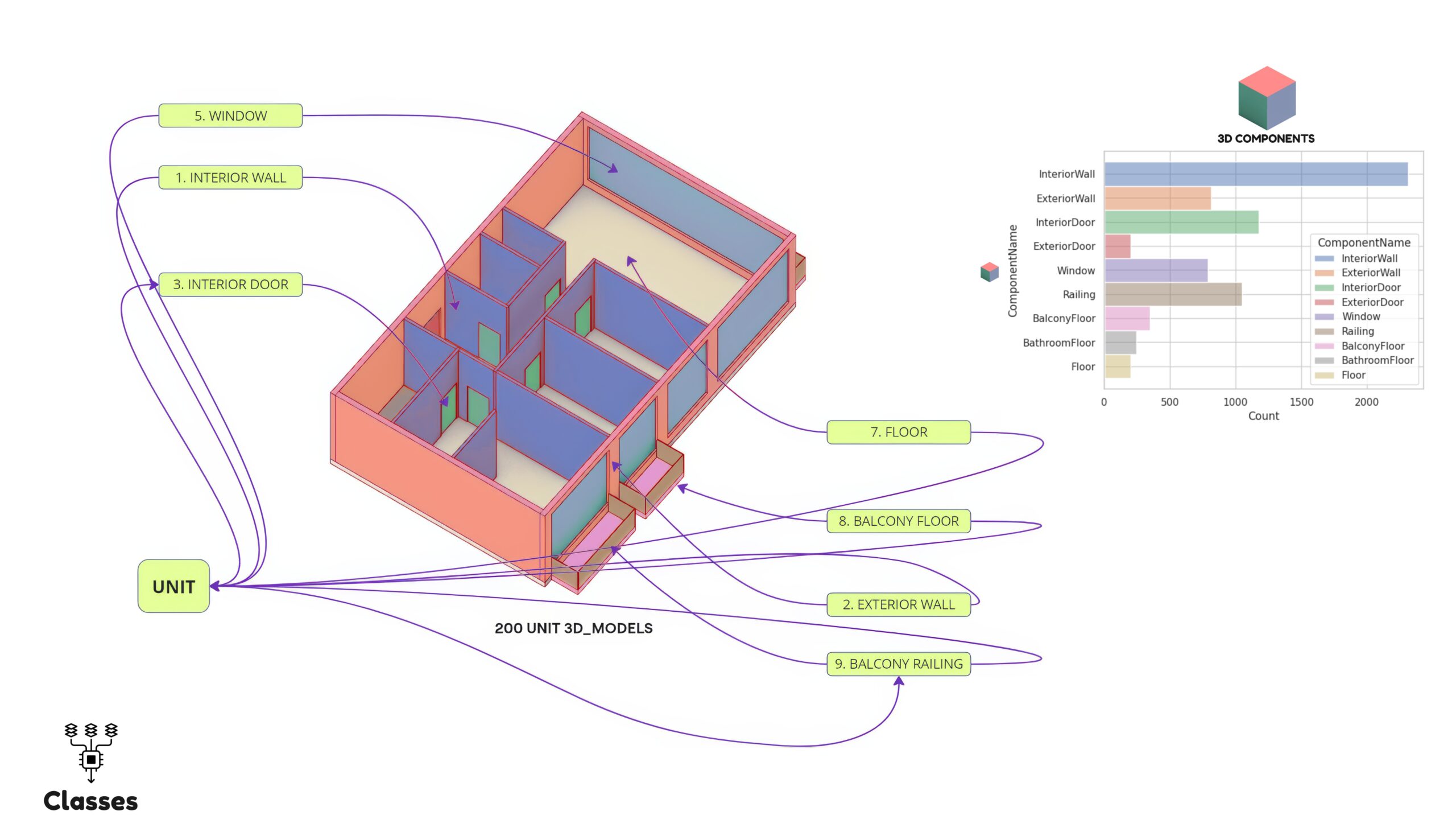
Components Breakdown
- 1. Interior Wall: Represented in blue, these form the internal structure of the unit.
- 2. Exterior Wall: Shown in red, these are the outer boundaries of the unit.
- 3. Interior Door: Marked in green, these facilitate movement within the unit.
- 5. Window: Indicated in purple, these elements contribute to natural lighting and ventilation.
- 7. Floor: Displayed in beige, forming the base of the unit.
- 8. Balcony Floor: Highlighted in orange, representing outdoor living spaces.
- 9. Balcony Railing: Shown in yellow, ensuring safety for balcony areas.
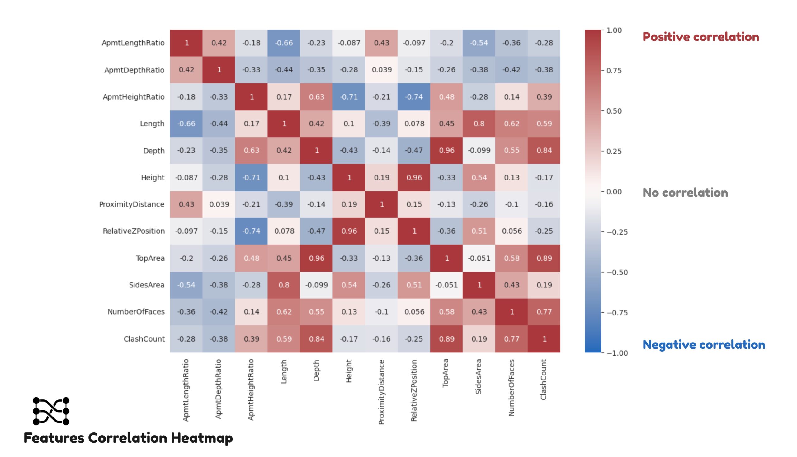
In our analysis, we identified several key features that play crucial roles in the urban planning framework. These features include the ratios of apartment length, depth, and height (AptmLengthRatio, AptmDepthRatio, AptmHeightRatio), as well as the physical dimensions of the components (Length, Depth, Height). ProximityDistance measures the distance to the nearest neighboring component, while RelativeZPosition indicates the vertical positioning relative to other components. The surface areas of the top and sides of the components (TopArea, SidesArea), the number of faces each component has (NumberOfFaces), and the number of clashes detected with other components (ClashCount) were also important factors.
To reduce the complexity of our dataset and capture the most variance, we derived six principal components (PC1 to PC6) from these features. Each principal component represents a combination of features that explains the maximum variance. In interpreting the principal components, correlation values were color-coded: red for positive correlations, blue for negative correlations, and neutral for little to no correlation. This color-coding helps in understanding how each feature contributes to the principal components.
Our insights revealed that the AptmDepthRatio shows a strong correlation with PC1, indicating its significant influence in this component. ProximityDistance is highly correlated with PC3, suggesting its importance in spatial arrangements. Additionally, ClashCount has a significant positive correlation with PC1, highlighting its impact on the primary principal component.
The “Features by Classes” slide visualizes how the 3D-SOLIDS Component Classification tool distributes various architectural components based on individual features. Scatter plots show the distribution of components like InteriorWall, ExteriorWall, Window, and Door across different features such as Length, Depth, Height, and ProximityDistance. Each dot represents a data point, color-coded by component type. This visualization helps in understanding if a single feature can effectively separate different components, aiding in accurate and efficient classification.
Features in Pairs: Analyzing Architectural Components: The “Features in Pairs” slide showcases how the 3D-SOLIDS Component Classification tool uses various feature combinations to distinguish between different architectural components effectively. Scatter plots illustrate relationships between features like Length, Depth, Apartment Depth Ratio, Height, Proximity Distance, and Relative Z Position. Each dot represents a specific data point for an architectural component, color-coded for different types (e.g., InteriorWall, ExteriorWall, Window). Red circles highlight significant clusters, such as distinct groups in Length vs. Depth and Apartment Depth Ratio vs. Height plots, indicating how features help classify components. The pair plot further demonstrates the clear separation of components using Apartment Depth and Height Ratios.
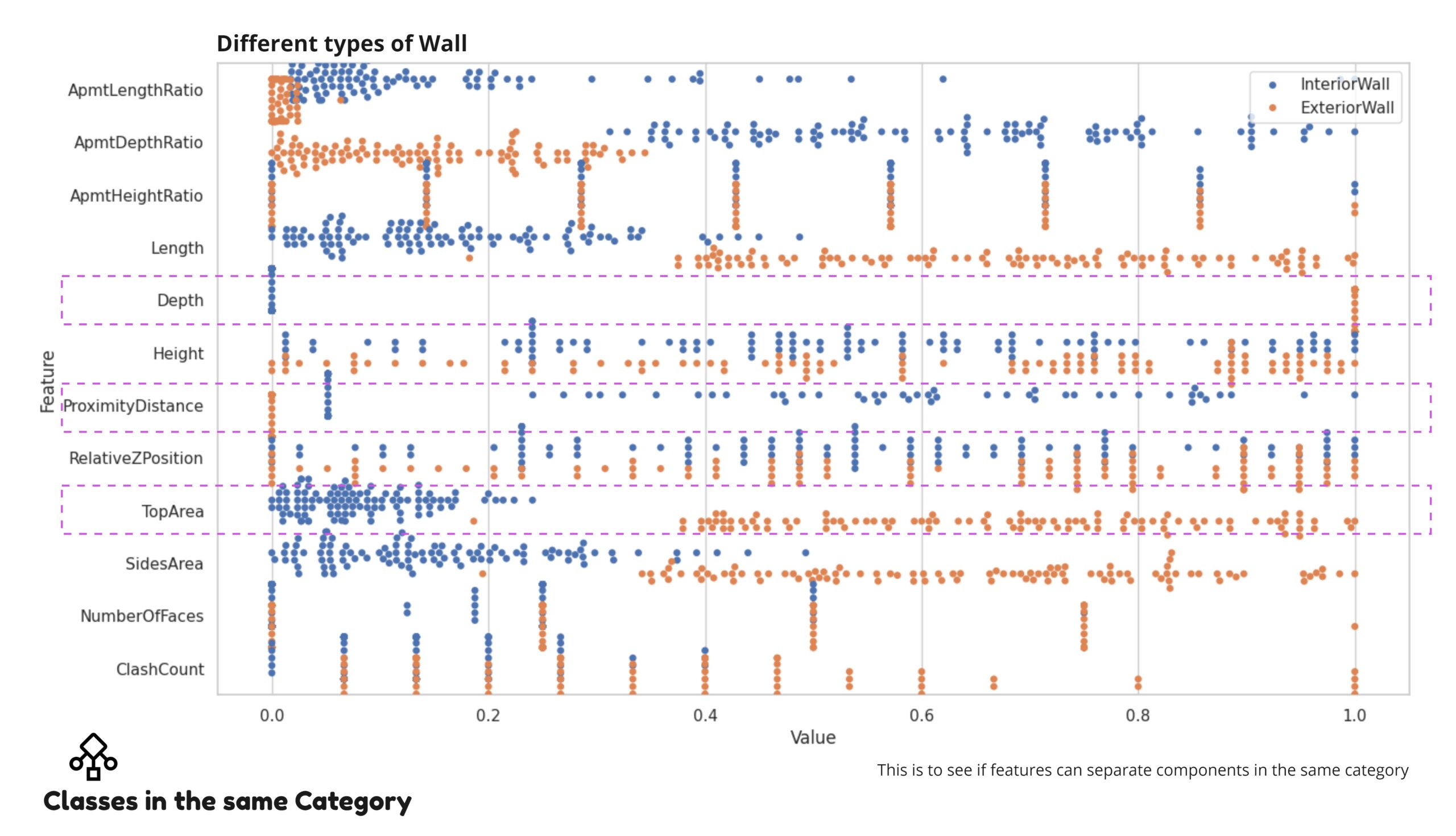
The “Classes in the Same Category” slide demonstrates how the 3D-SOLIDS Component Classification tool distinguishes between InteriorWall and ExteriorWall using various features. The scatter plot shows the distribution of these wall types across features like Length, Depth, Height, and ProximityDistance, with blue dots representing InteriorWalls and orange dots representing ExteriorWalls. The distinct patterns and separations highlighted by purple dashed lines indicate how specific features can effectively classify components within the same category. This precise feature-based analysis enhances the tool’s ability to automate and optimize architectural design processes.
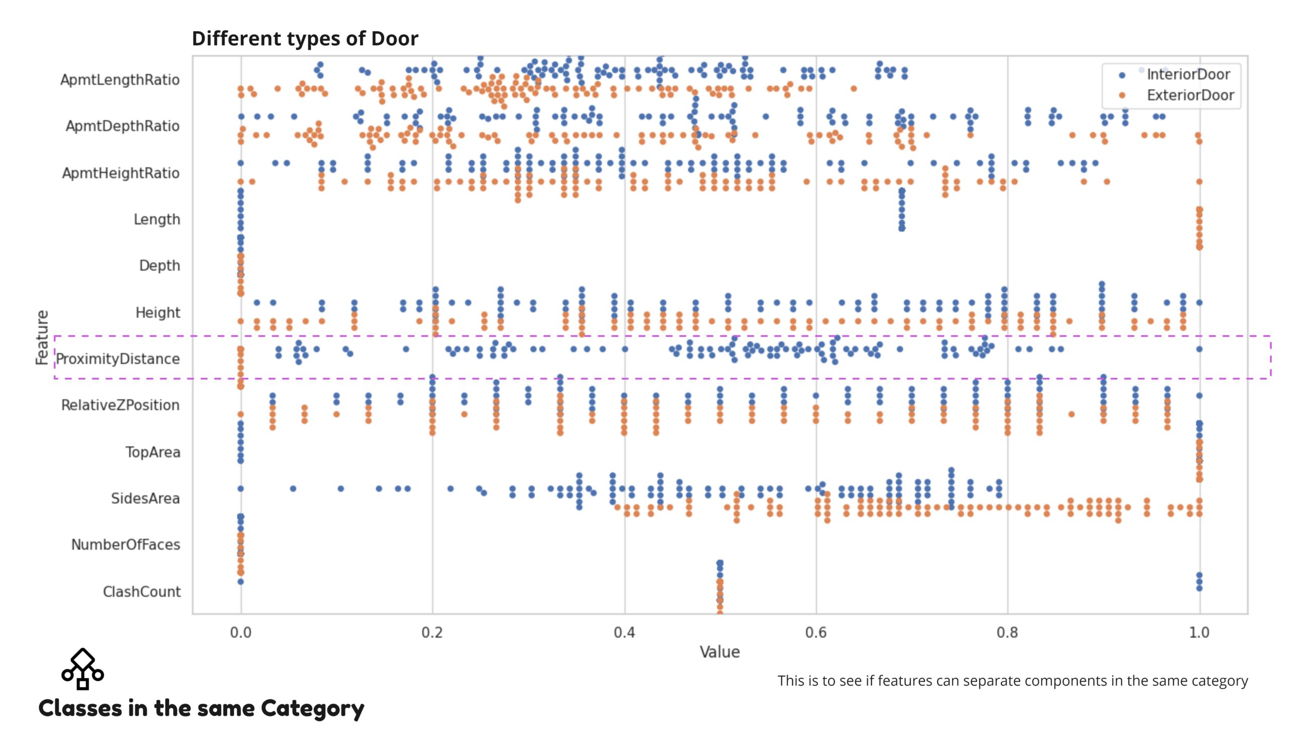
The “Classes in the Same Category” slide highlights how the 3D-SOLIDS Component Classification tool distinguishes between InteriorDoor and ExteriorDoor using various features. The scatter plot shows the distribution of these door types across features like Length, Depth, Height, and ProximityDistance, with blue dots representing InteriorDoors and orange dots representing ExteriorDoors. The clear separation along ProximityDistance (highlighted by the purple dashed line) indicates the effectiveness of this feature in classifying doors within the same category, enhancing design accuracy and efficiency.
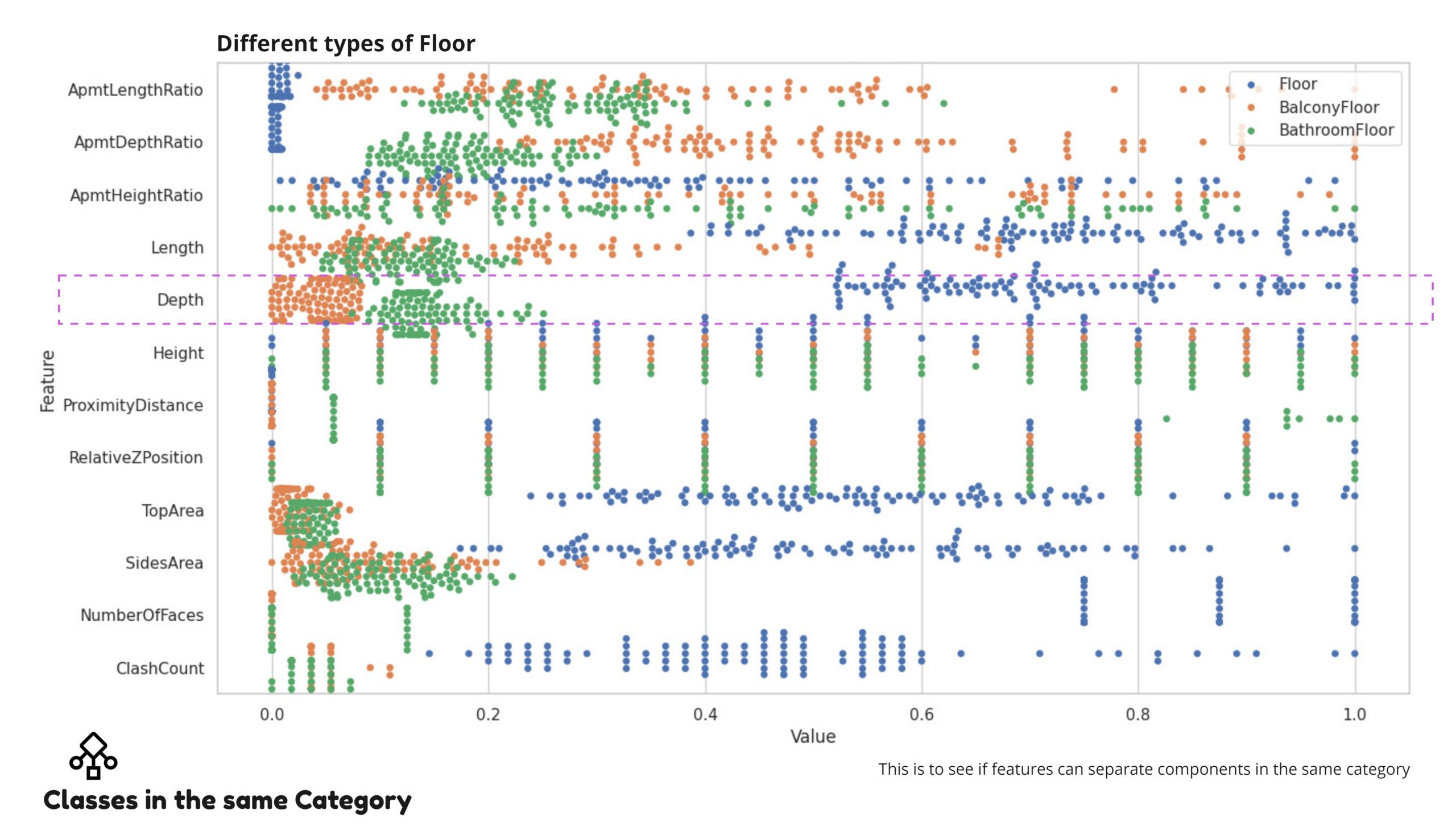
The “Classes in the Same Category” slide illustrates how the 3D-SOLIDS Component Classification tool differentiates between Floor, BalconyFloor, and BathroomFloor using various features. The scatter plot shows the distribution of these floor types across features like Length, Depth, Height, and ProximityDistance, with blue, orange, and green dots representing different floor types. The distinct clustering along the Depth feature (highlighted by the purple dashed line) demonstrates its effectiveness in classifying floor components within the same category, enhancing design precision and efficiency.
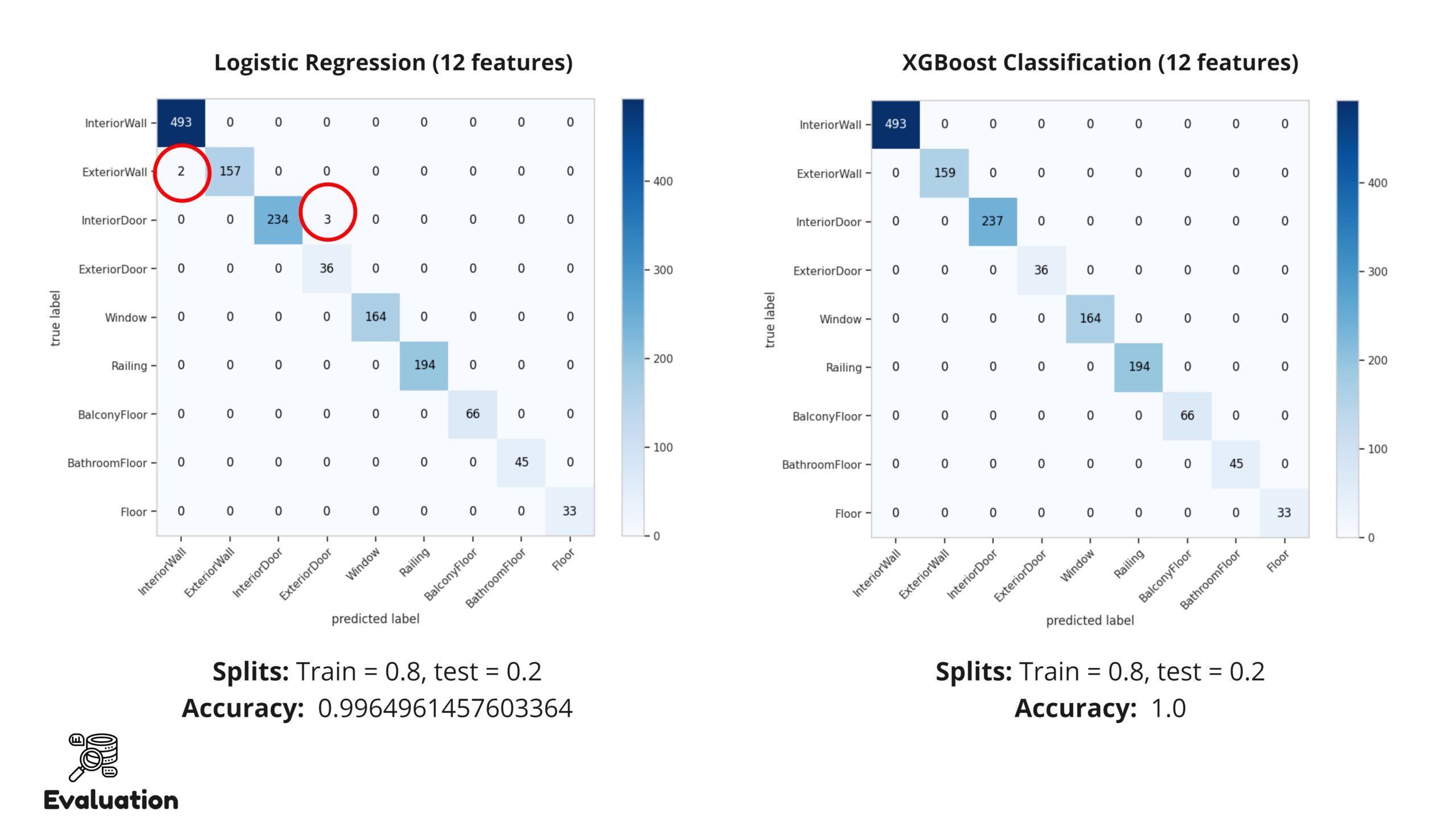
The evaluation slide compares the performance of Logistic Regression and XGBoost Classification models in identifying architectural components. The Logistic Regression model, with a train-test split of 80%-20%, achieved an accuracy of 99.65%, showing minor misclassifications in ExteriorWall and InteriorDoor. In contrast, the XGBoost Classification model, using the same data split, achieved perfect accuracy with no misclassifications. The XGBoost’s superior capability in accurately classifying architectural elements.
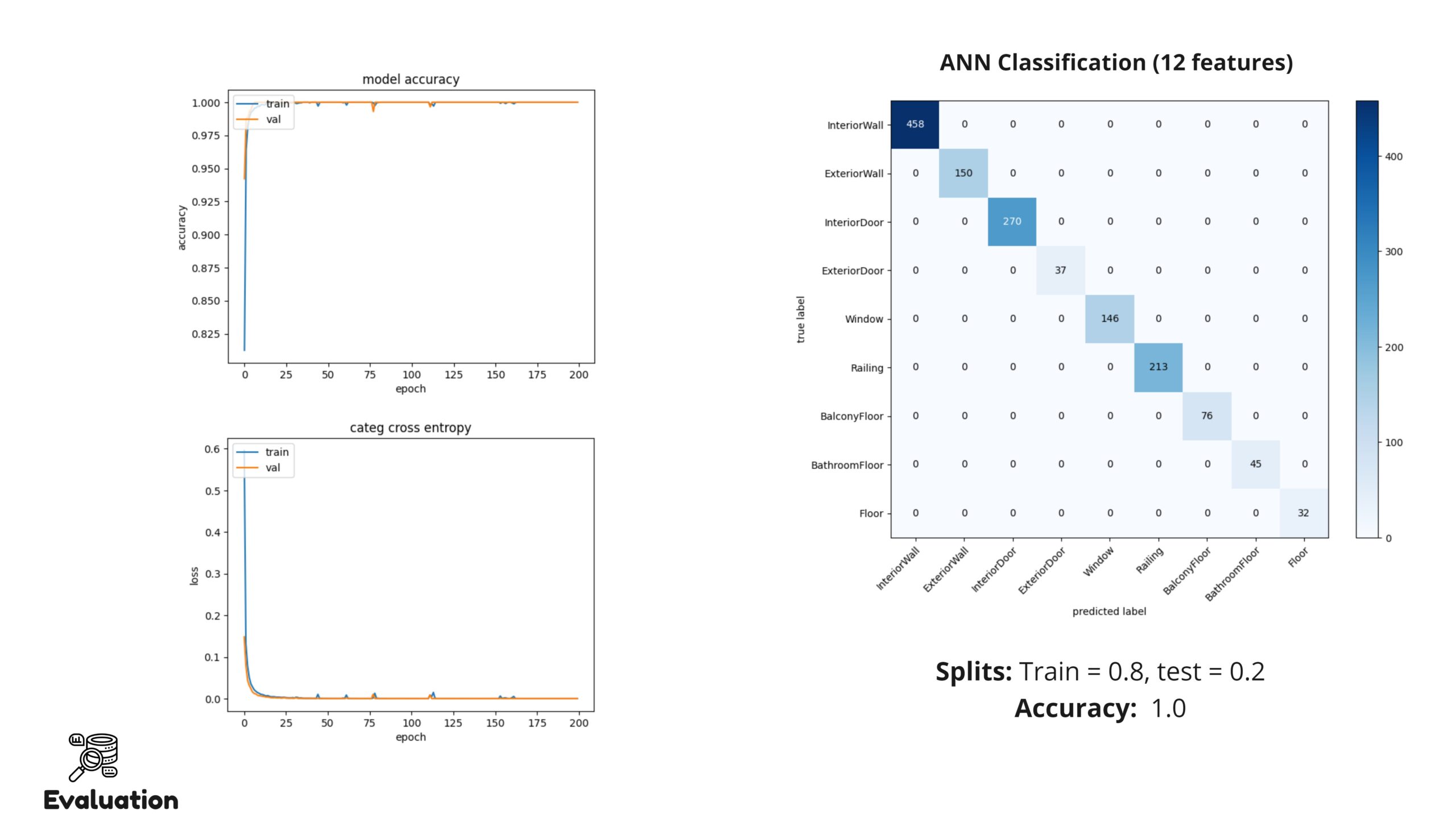
The slide presents the evaluation of an Artificial Neural Network (ANN) model using 12 features to classify architectural components. The model achieved perfect accuracy (100%) with an 80%-20% train-test split. The confusion matrix shows precise classification across all component types, with no misclassifications. The accompanying plots of model accuracy and categorical cross-entropy loss over 200 epochs indicate robust training performance, with both training and validation metrics converging effectively. The ANN model’s superior performance and reliability in classifying architectural elements.
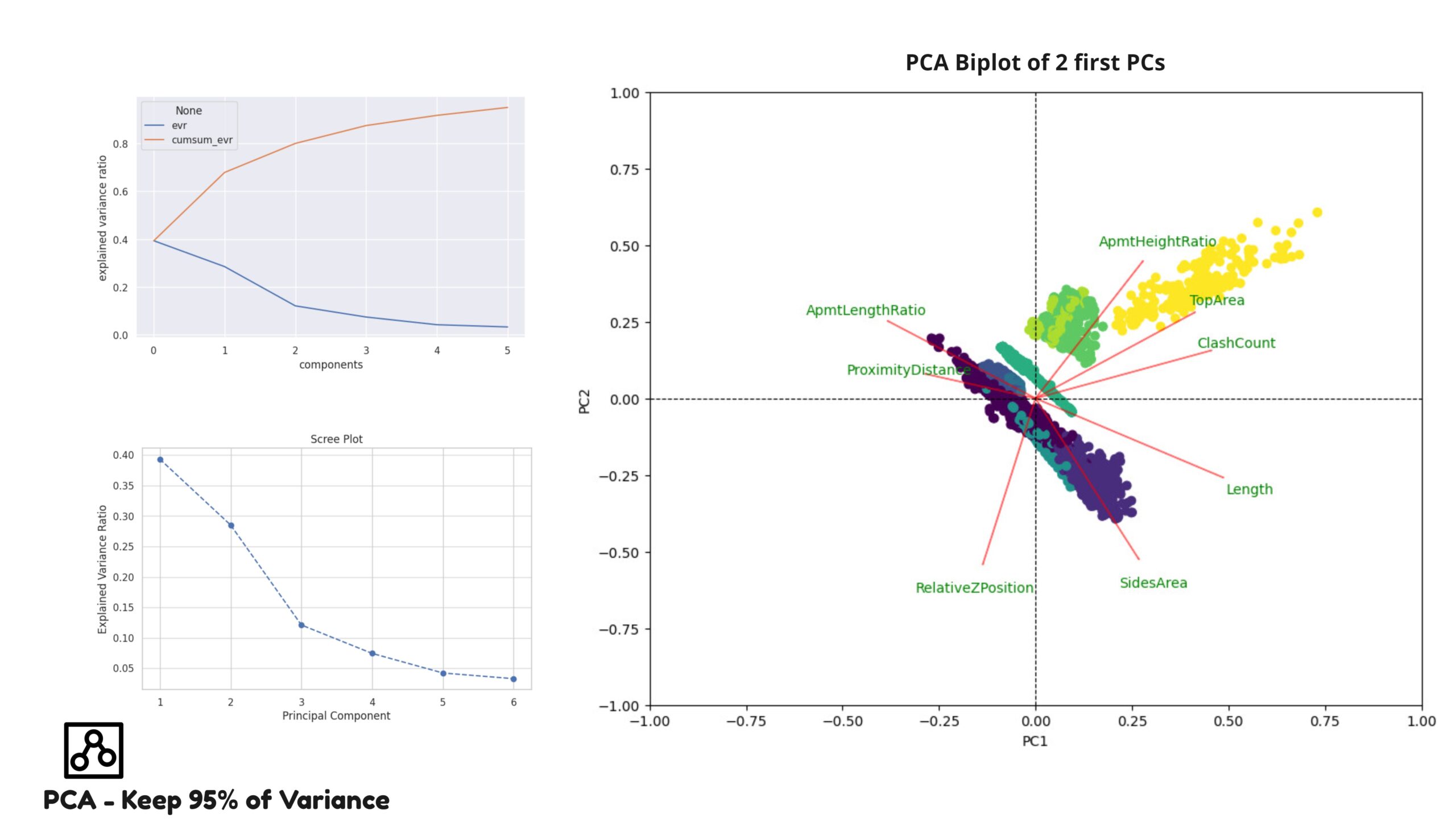
The “PCA: Keep 95% of Variance” slide illustrates how Principal Component Analysis (PCA) is used to reduce dimensionality while retaining 95% of the data’s variance. The explained variance ratio plot shows how much variance is captured by each principal component, with the cumulative variance indicating that the first few components capture most of the variance. The scree plot highlights the explained variance for each principal component, helping to identify the optimal number of components. The PCA biplot visualizes the first two principal components (PC1 and PC2), showing the influence of features like Length, Depth, and ProximityDistance. The distinct clusters in the biplot indicate clear groupings of architectural elements, enhancing the tool’s ability to classify components effectively and efficiently. This dimensionality reduction ensures accurate classification while simplifying the computational process.
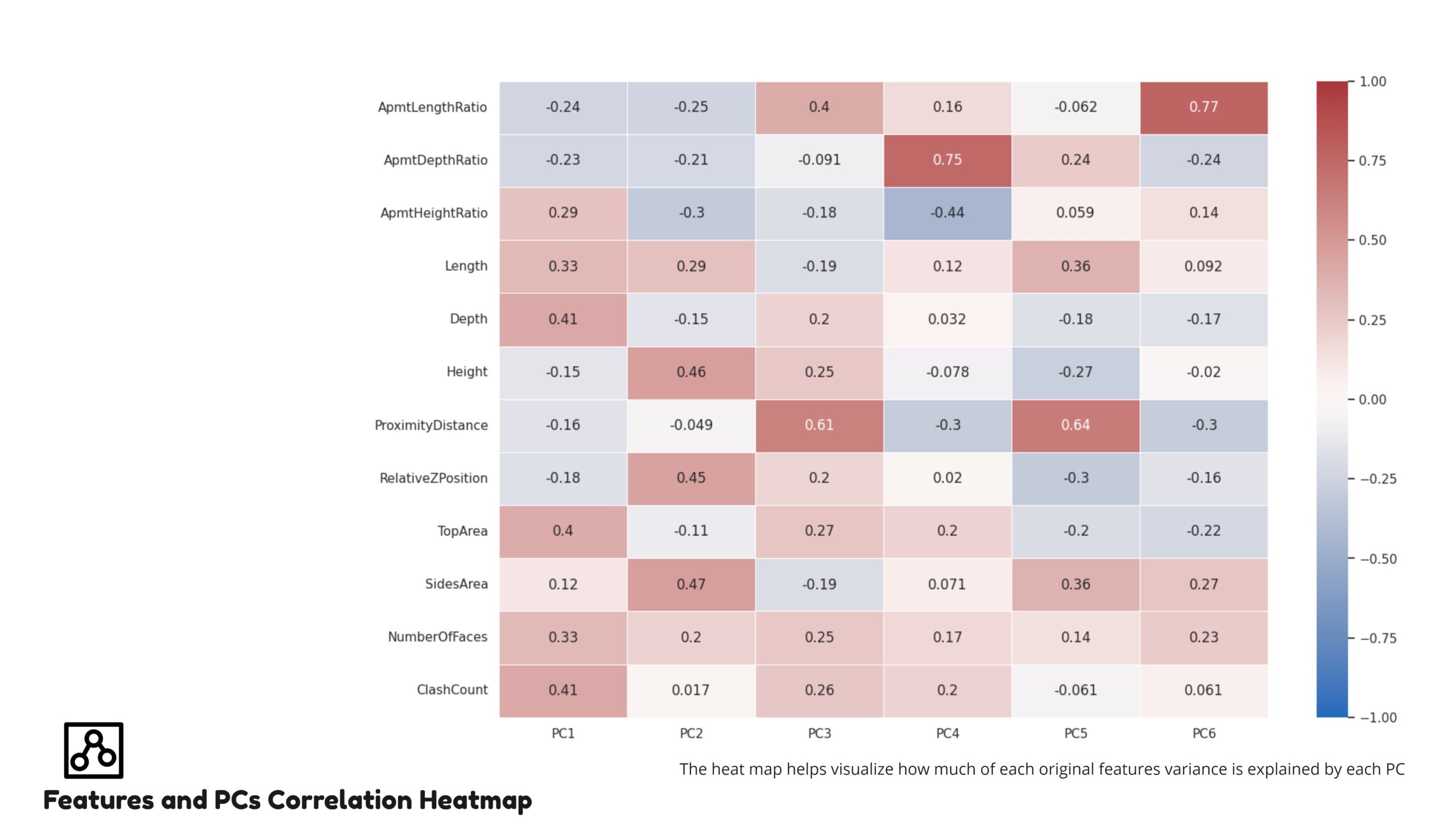
The “Features and PCs Correlation Heatmap” slide illustrates the relationship between original features and principal components (PCs) in the 3D-SOLIDS Component Classification tool. The heatmap shows how much variance of each feature is explained by each PC, with color intensity indicating the strength and direction of the correlation. For instance, features like ApartmentDepthRatio and ProximityDistance show strong positive correlations with specific PCs, while others like Height and RelativeZPosition exhibit varied correlations across multiple PCs.
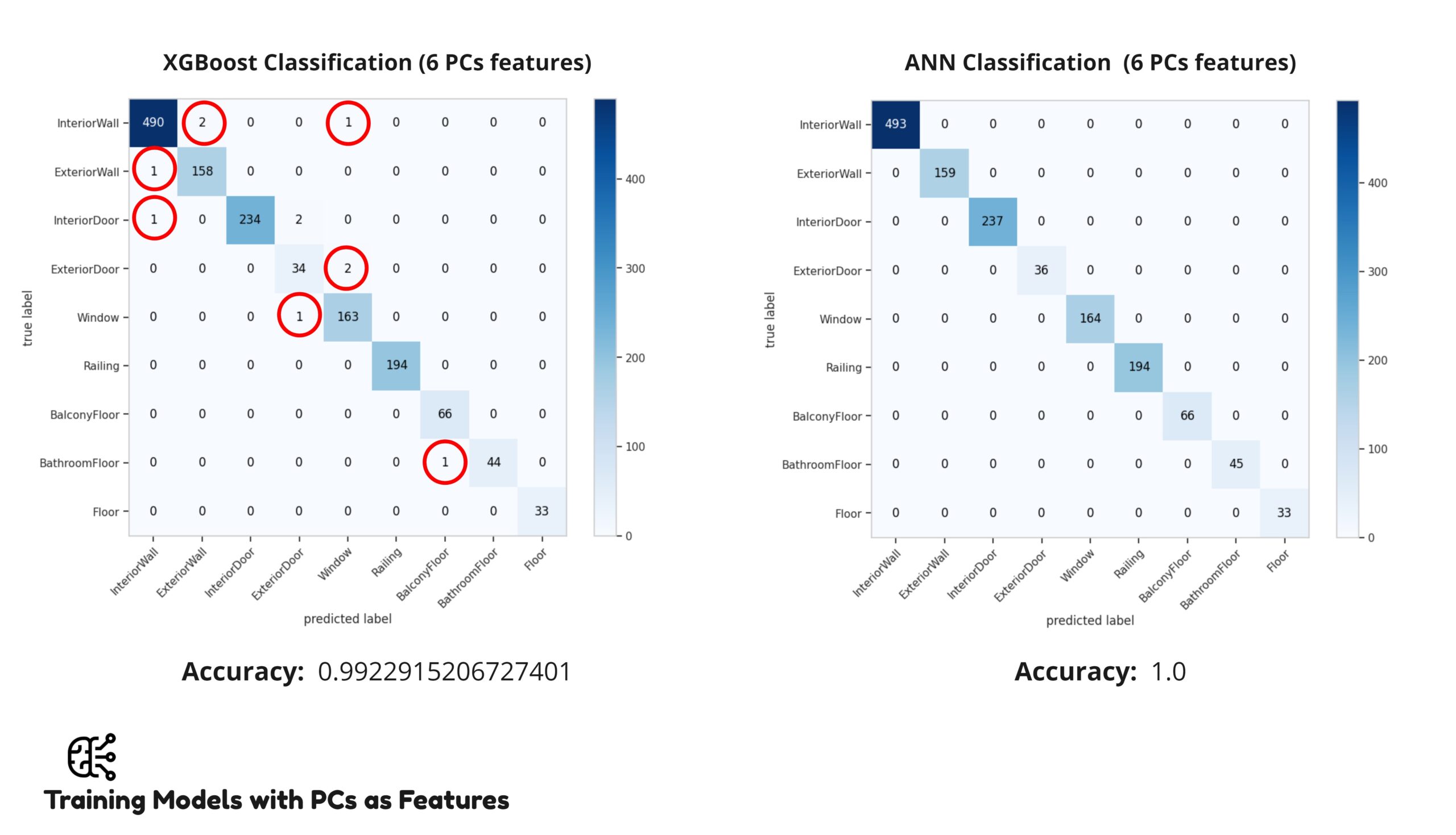
The “Training Models with PCs as Features” slide compares the performance of XGBoost and ANN models using principal components (PCs) for feature classification. The XGBoost model, using six PCs, achieved an accuracy of 99.23%, with minor misclassifications highlighted in the confusion matrix. In contrast, the ANN model also utilized six PCs but achieved perfect classification with an accuracy of 100%, showing no misclassifications.
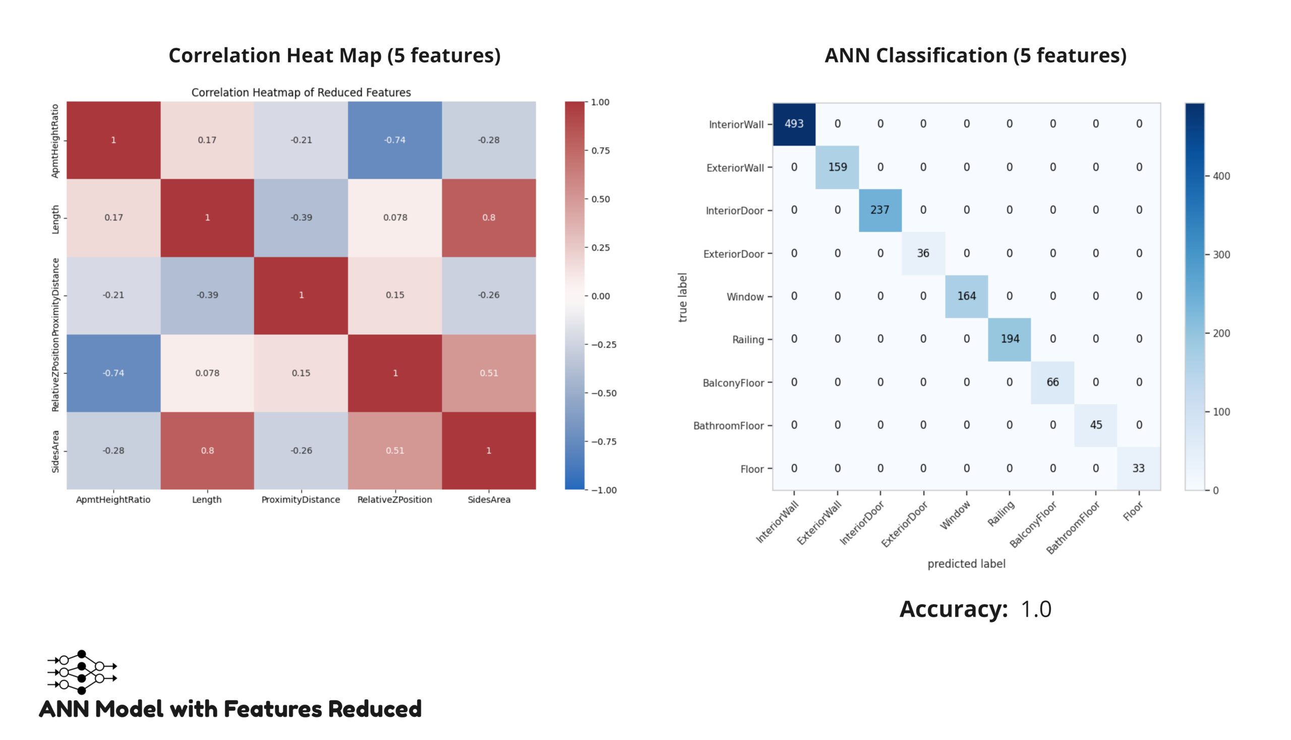
The “ANN Model with Features Reduced” slide evaluates the performance of an Artificial Neural Network (ANN) model using a reduced set of five features. The correlation heatmap shows the relationships between the selected features (ApartmentHeightRatio, Length, ProximityDistance, RelativeZPosition, and SidesArea), indicating their contribution to the model. The confusion matrix demonstrates perfect classification across all architectural components, with the model achieving an accuracy of 100%. This reduction in features, while maintaining high accuracy, highlights the model’s efficiency and effectiveness in classifying components with a simplified feature set.
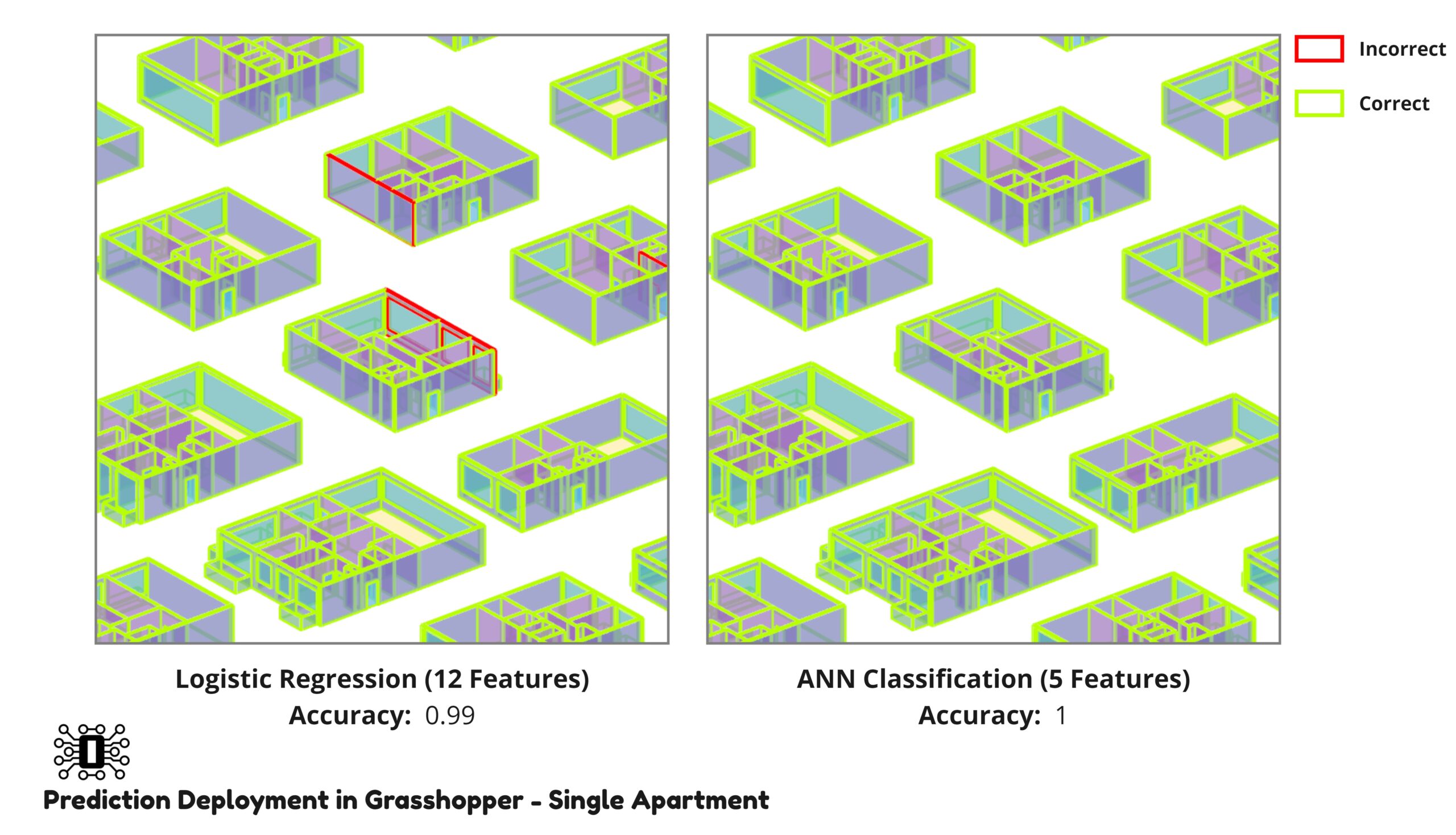
The “Prediction Deployment in Grasshopper – Single Apartment” slide demonstrates the application of predictive models within a 3D modeling environment, specifically comparing Logistic Regression and ANN models. The Logistic Regression model, utilizing 12 features, achieved an accuracy of 99%, with a few incorrect classifications highlighted in red. In contrast, the ANN model, using only 5 features, achieved perfect accuracy, with all components correctly classified in green.
The “Prediction Deployment in Grasshopper – Single Apartment” slide showcases the effectiveness of predictive models within a 3D modeling environment. The Logistic Regression model, using 12 features, achieved an accuracy of 99% but displayed some incorrect classifications, as highlighted in red, where an InteriorWall was misclassified as an ExteriorWall. In contrast, the ANN model, using only 5 features, achieved perfect accuracy with all classifications correct, shown in green.
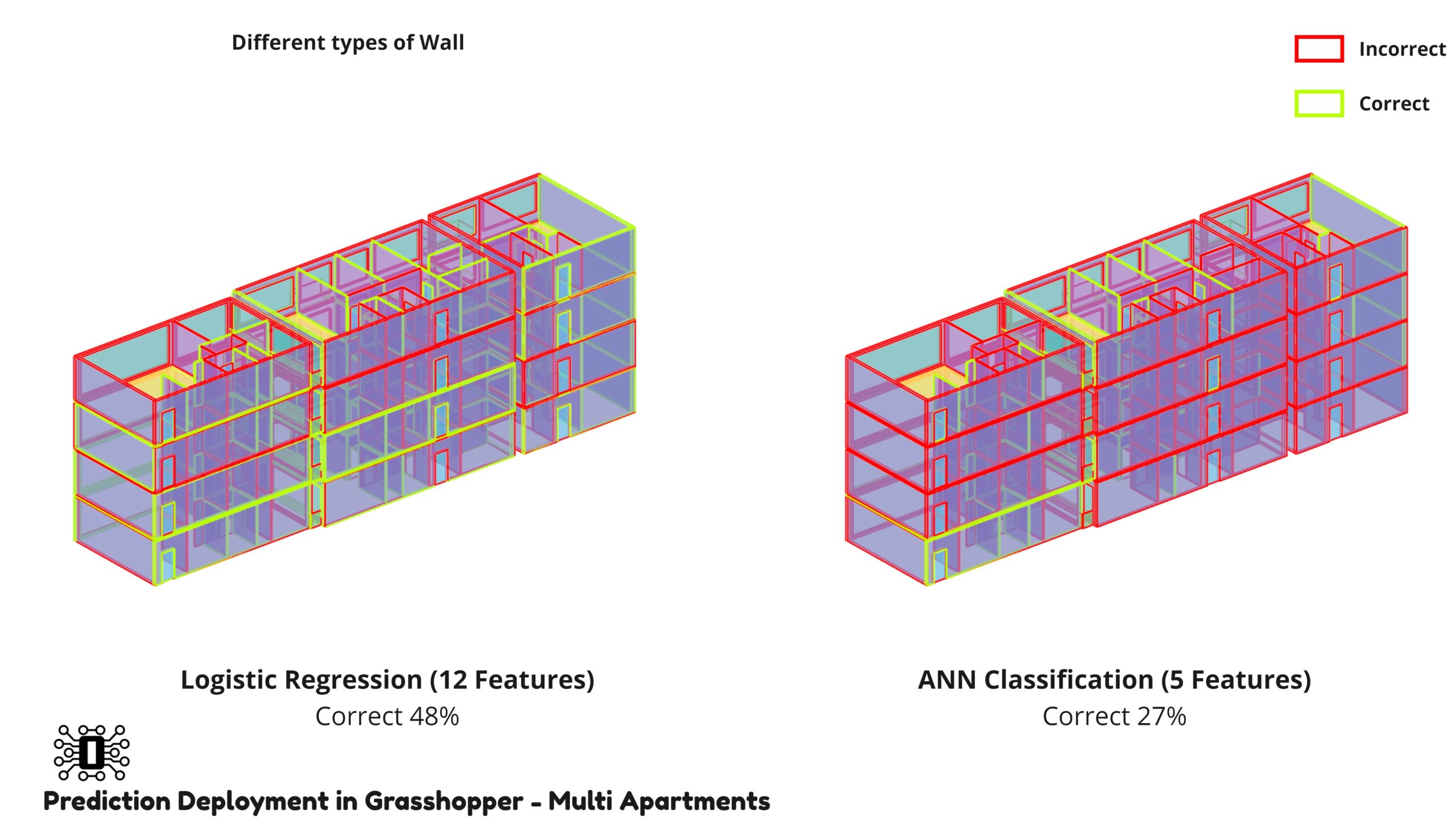
The “Prediction Deployment in Grasshopper – Multi Apartments” slide evaluates the performance of Logistic Regression and ANN models in a multi-apartment setting. The Logistic Regression model, using 12 features, correctly classified 48% of the components, with incorrect classifications highlighted in red. The ANN model, using only 5 features, achieved a lower correct classification rate of 27%. The high number of incorrect classifications in both models indicates the increased complexity and challenges of predicting components accurately in multi-apartment structures, highlighting the need for further model refinement and feature enhancement for complex architectural scenarios.
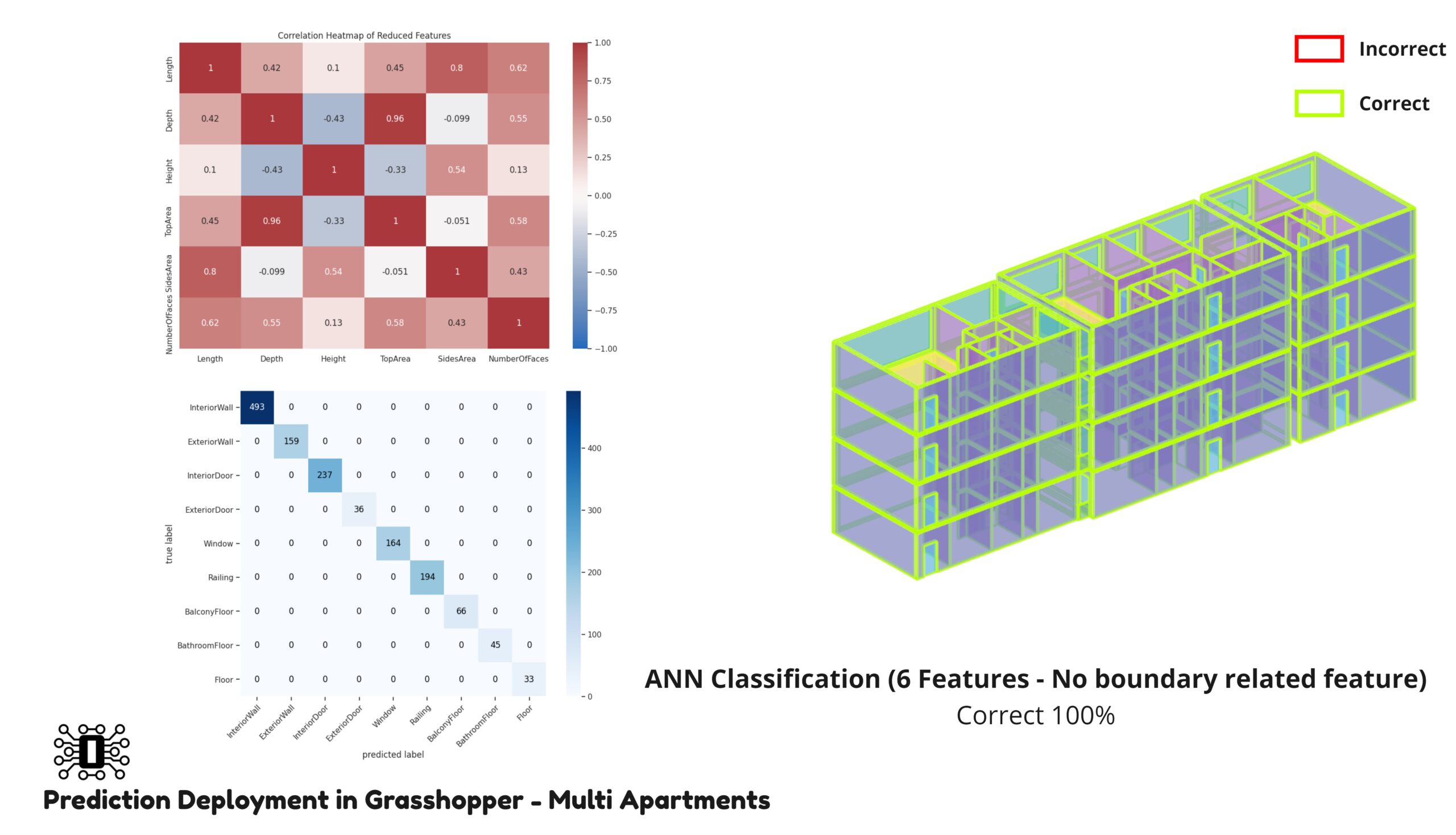
The “Prediction Deployment in Grasshopper – Multi Apartments” slide showcases the performance of an ANN model using six features, excluding boundary-related features, for classifying components in a multi-apartment structure. The correlation heatmap displays the relationships between the reduced features, while the confusion matrix shows perfect classification with no errors.
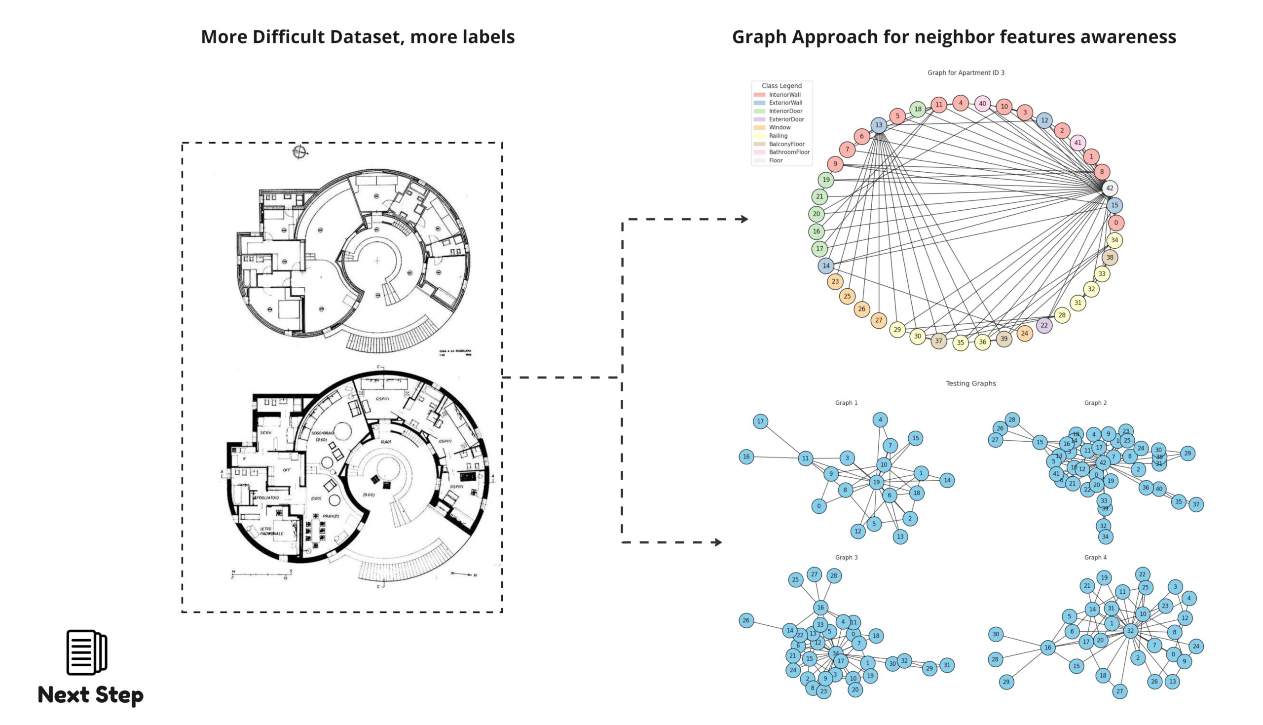
More Difficult Dataset, More Labels:
- The left image depicts more complex floor plans with additional labels, indicating the need to handle more intricate datasets in future developments.
Graph Approach for Neighbor Features Awareness:
- The right side introduces a graph-based approach to account for neighbor feature relationships, enhancing classification accuracy.
- The circular graph shows the interconnections between different components within an apartment.
- The smaller graphs illustrate various testing scenarios, emphasizing the importance of understanding spatial relationships and connectivity.
AIA Data Encoding Seminar
Project Team:
- Bao Q. Trinh
- Manolya Nielsen
- Hetal Bharwanu
- Agustin Salas
3D-SOLIDS: COMPONENTS CLASSIFICATION is a project of Iaac, Institute for Advanced Architecture of Catalonia developed at Master in Advanced Computation for Architecture & Design in 2023-24 by Students: Bao Q. Trinh, Manolya Nielsen, Hetal Bharwanu and Agustin Salas, under the supervision of Faculty: @Gabriella Rossi, Georgios Bekakos, Panayota Pouliou.
