
Introduction
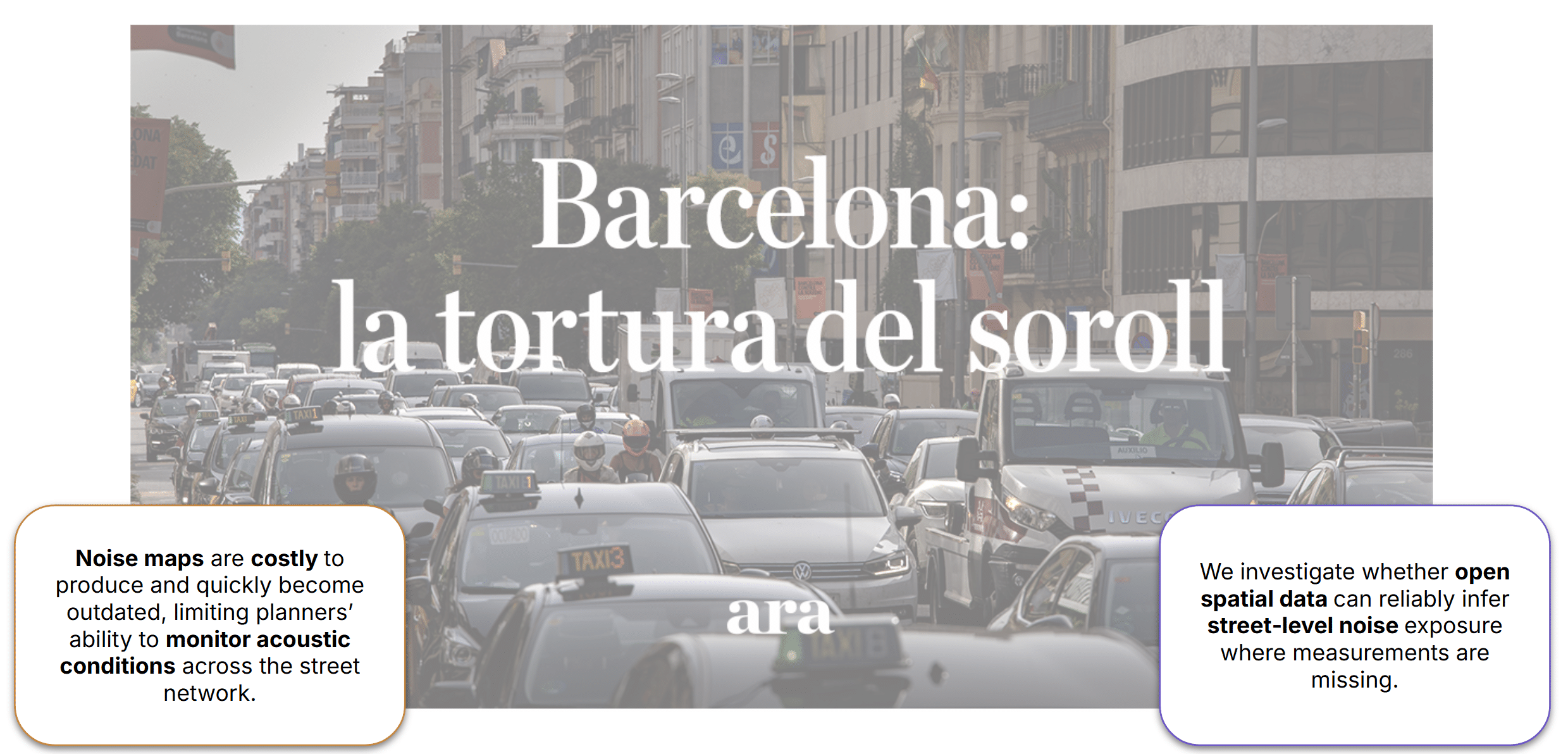
Noise is one of the most pervasive environmental stressors in cities. Long-term exposure has been linked to sleep disturbance, cardiovascular disease, reduced cognitive performance, and lower overall quality of life. Yet despite its importance, detailed noise maps are surprisingly difficult to obtain.
Producing official noise maps requires measurements, traffic models, and considerable technical effort. As a result, they are expensive to update and often unavailable in smaller cities. Even where they exist, they can quickly become outdated as traffic patterns and urban environments change.
This raises an interesting question:
Can we estimate street-level noise exposure using only openly available spatial data?
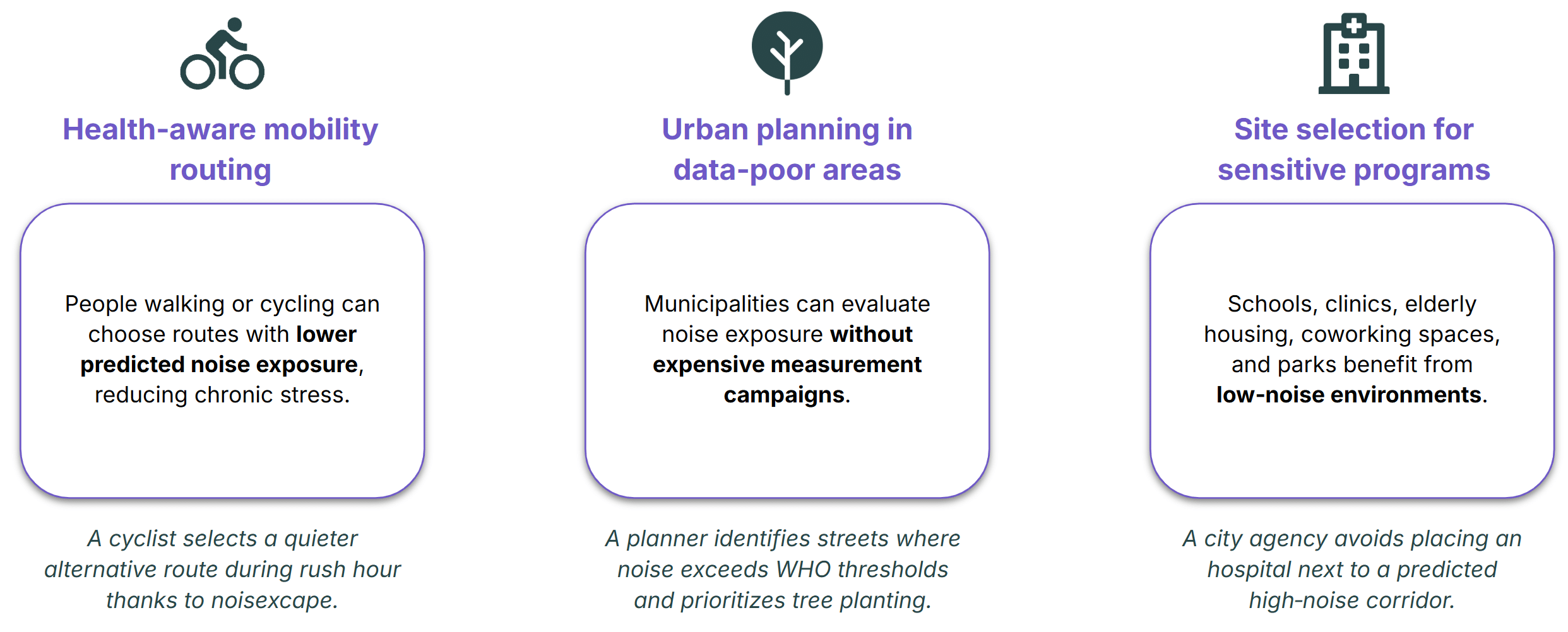
If the answer is yes, cities could monitor acoustic conditions more frequently and at a much lower cost. Such estimates could support applications ranging from health-aware routing and urban planning to the placement of noise-sensitive facilities such as schools and hospitals.
What Previous Studies Tell Us
A study conducted across five Bulgarian cities used machine learning models to estimate traffic noise from geometric and spatial features. One of the strongest predictors was the amount of major road infrastructure within a 100-meter radius, while Random Forest and XGBoost delivered the best performance.
Another study covering four Chilean cities repeatedly identified street category as the most important predictor of urban noise levels.
These findings suggest that the physical structure of a city may already contain much of the information needed to estimate environmental noise.
Building the Barcelona Dataset
To test this hypothesis, we chose Barcelona as our case study.
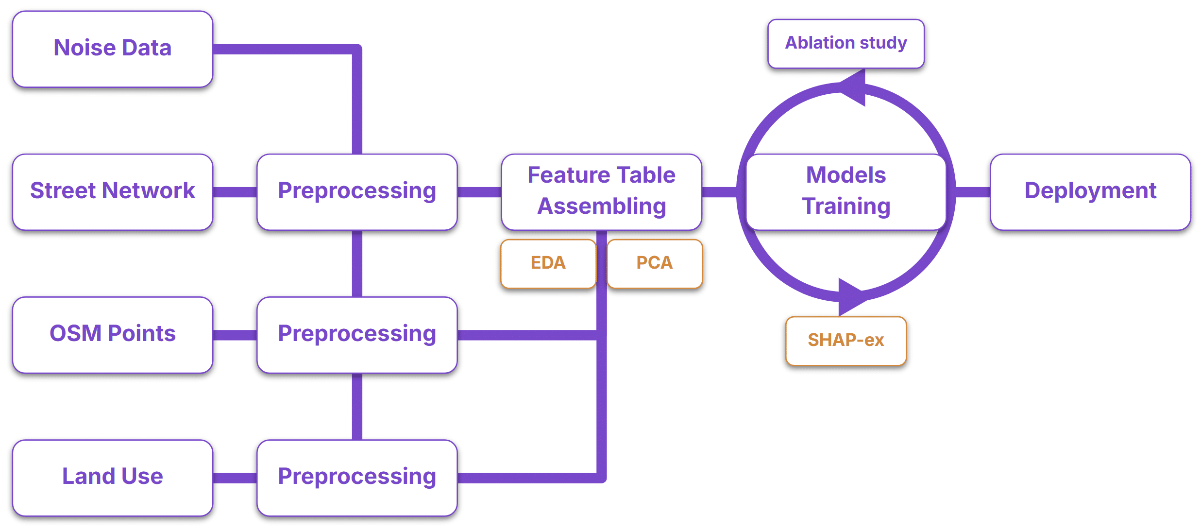
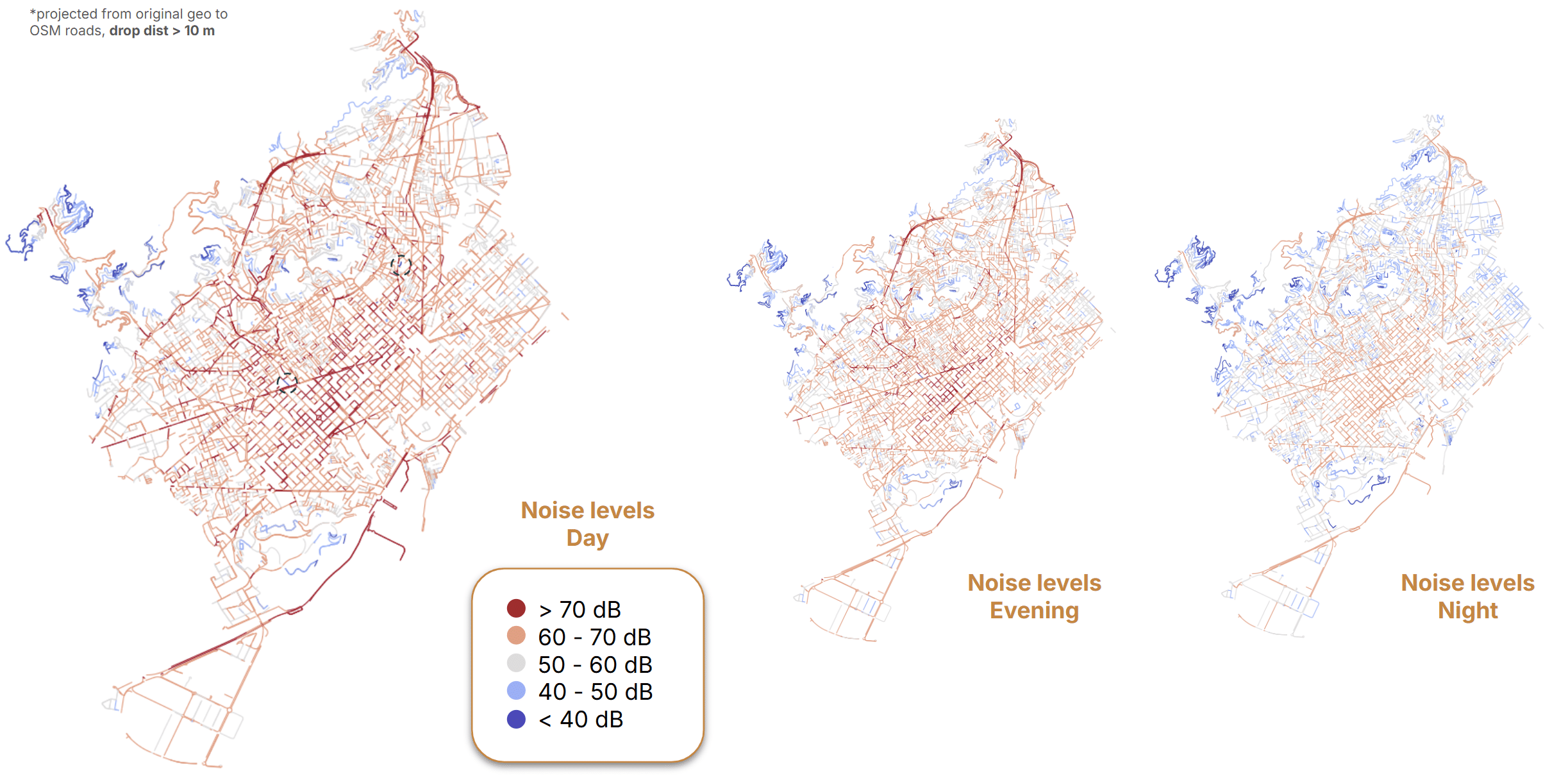
The target variable came from Barcelona’s open noise dataset, which provides day, evening, and night noise levels across the city. To build the predictor variables, we relied almost entirely on OpenStreetMap, extracting information about:
- Street networks
- Land use
- Public transport infrastructure
- Traffic signals
- Points of interest
Combining these datasets turned out to be less straightforward than expected.
The official noise map and the OpenStreetMap street network use different street segmentations. Before any analysis could begin, noise values had to be projected onto the OSM street network. To reduce matching errors, street segments whose nearest match exceeded 10 meters were removed.
We also performed several preprocessing steps:
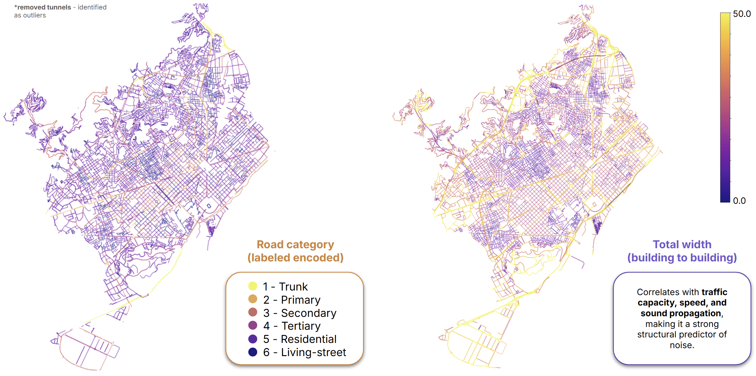
- Tunnel segments were removed because they behaved as outliers.
- Street categories were encoded as categorical variables
- Missing street-width information was replaced with a geometrically derived building-to-building distance metric.
After cleaning and harmonization, the dataset contained 12,854 street segments.
Describing the Urban Environment
One of the goals of this project was to understand how urban form influences noise.
To capture street-network structure, we included several space syntax metrics:
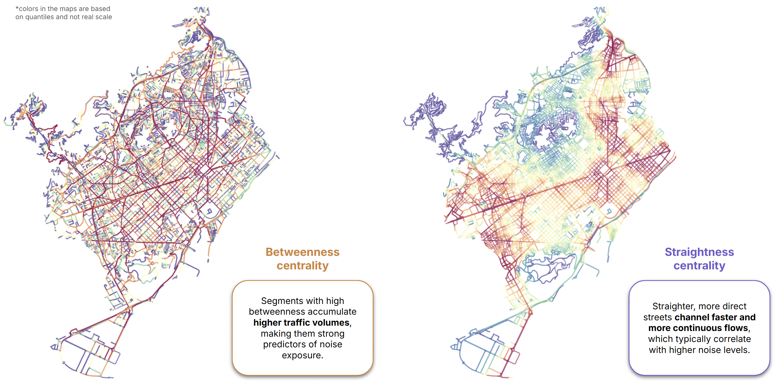
- Betweenness centrality, often used as a proxy for traffic volumes.
- Straightness centrality, which measures route directness.
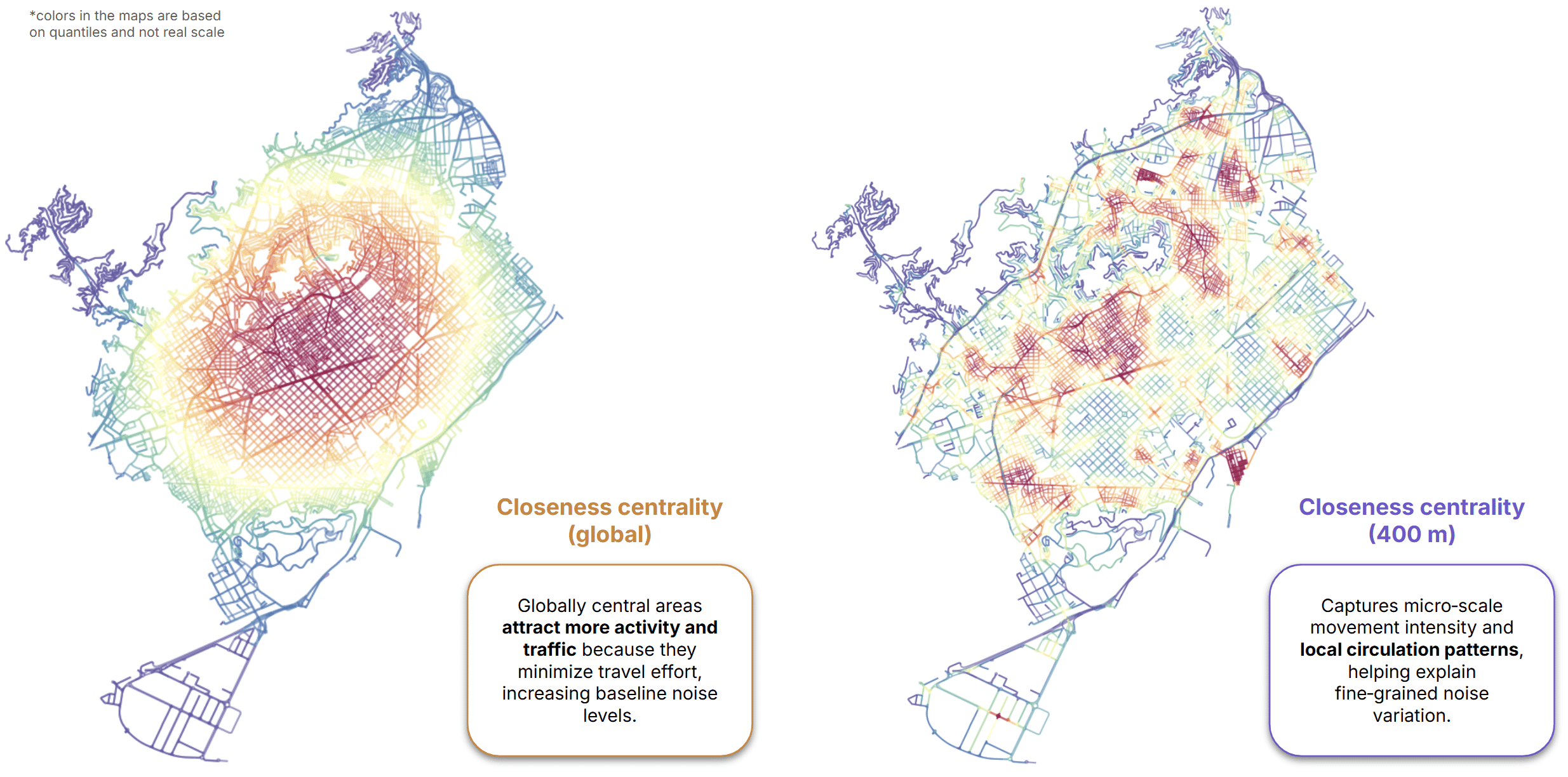
- Global closeness centrality, describing city-wide accessibility.
- Local closeness centrality, capturing neighborhood-scale accessibility.
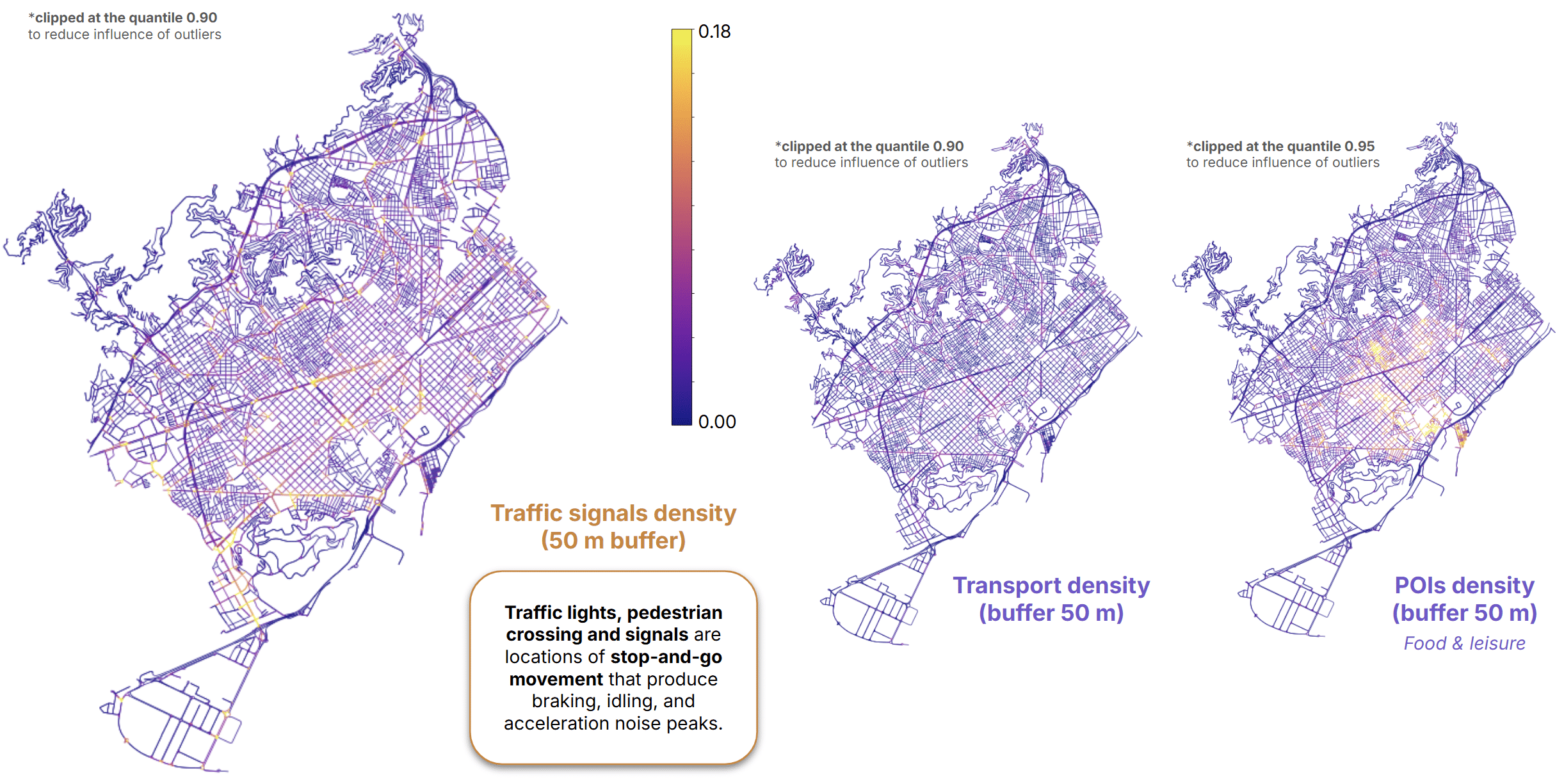
We also characterized the immediate surroundings of each street segment using a 50-meter buffer.
Within this area, we measured:
- Density of traffic signals
- Density of transport facilities
- Density of food and leisure activities
- Percentage of green land use
- Percentage of commercial land use
- Percentage of industrial land use
Finally, we included distance-based measures to different road categories.
The resulting feature space consisted of 18 variables.
First Look at the Data – EDA & PCA
Before training any machine learning models, we wanted to understand what the data were telling us.
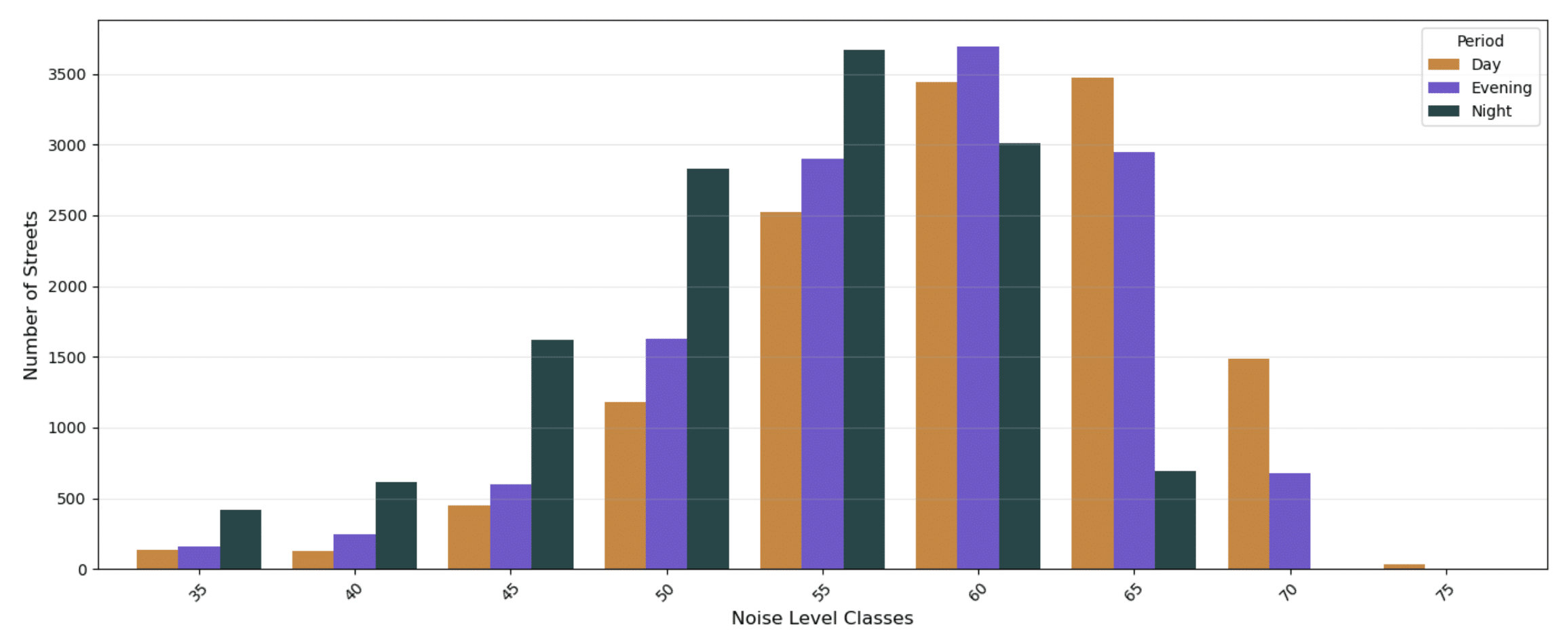
The distribution of noise levels was approximately Gaussian, although slightly more concentrated around the mean than a standard normal distribution. Unsurprisingly, the highest noise levels were largely absent from nighttime observations.
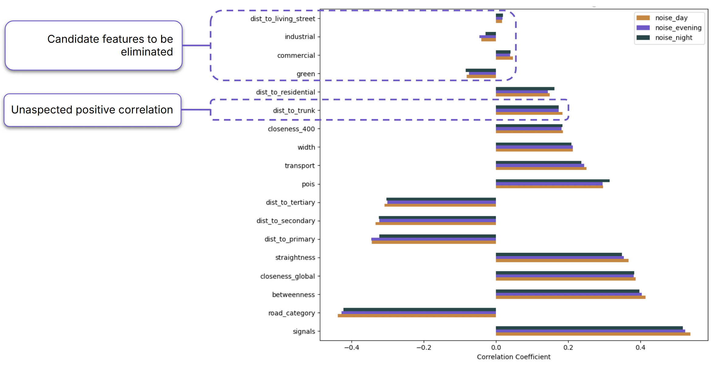
Looking at Spearman correlation between noise and predictors, one particularly interesting finding was an unexpected positive correlation between distance to trunk roads and noise levels. At the same time, some variables appeared to carry little information on their own. For example, land-use features and distance to living streets showed only weak correlations with noise.
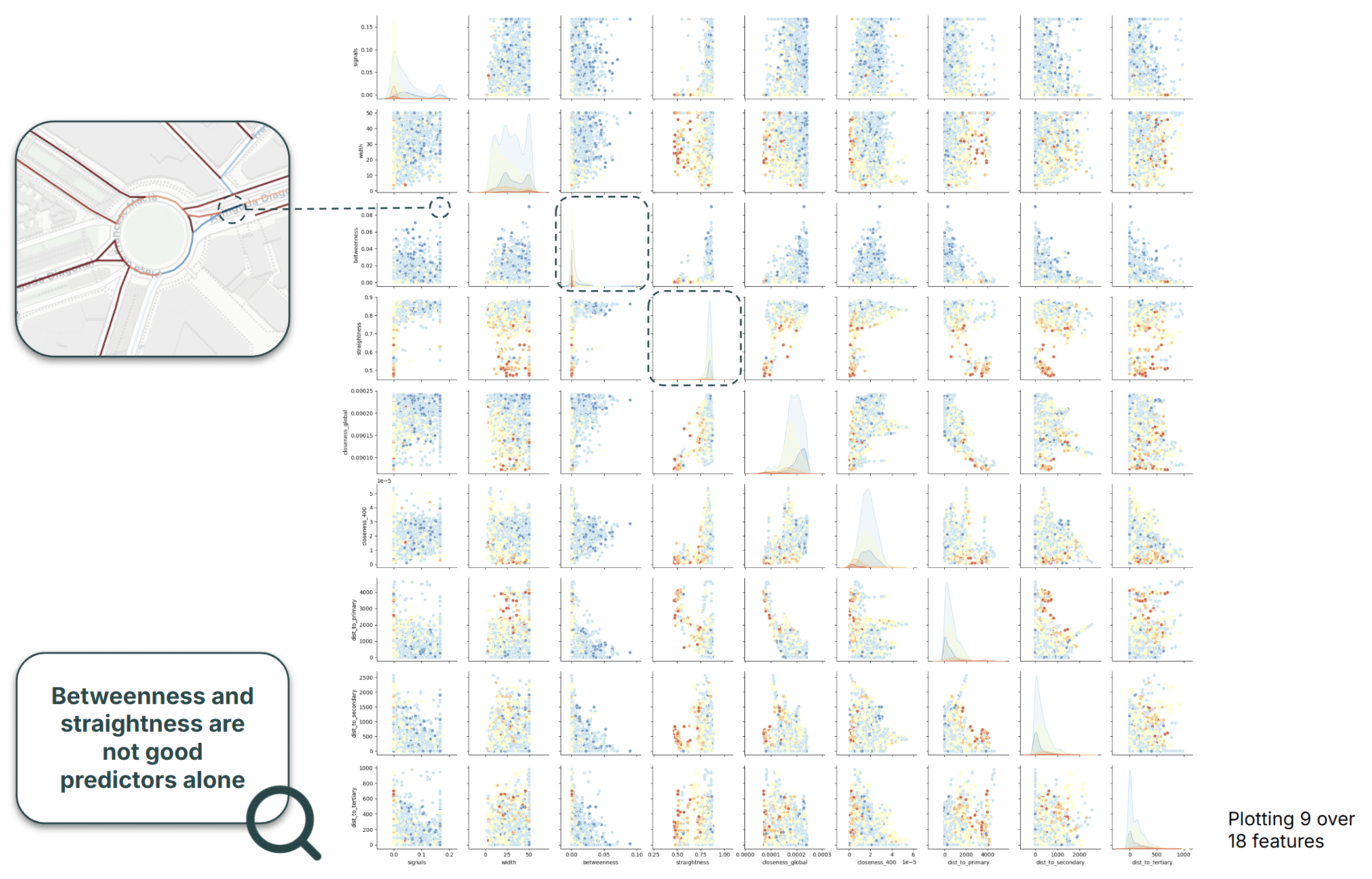
Pair plots revealed another interesting pattern: space syntax metrics such as betweenness and straightness centrality did not appear to be strong predictors when considered individually. This hinted that their value might emerge only when combined with other features through machine-learning models.
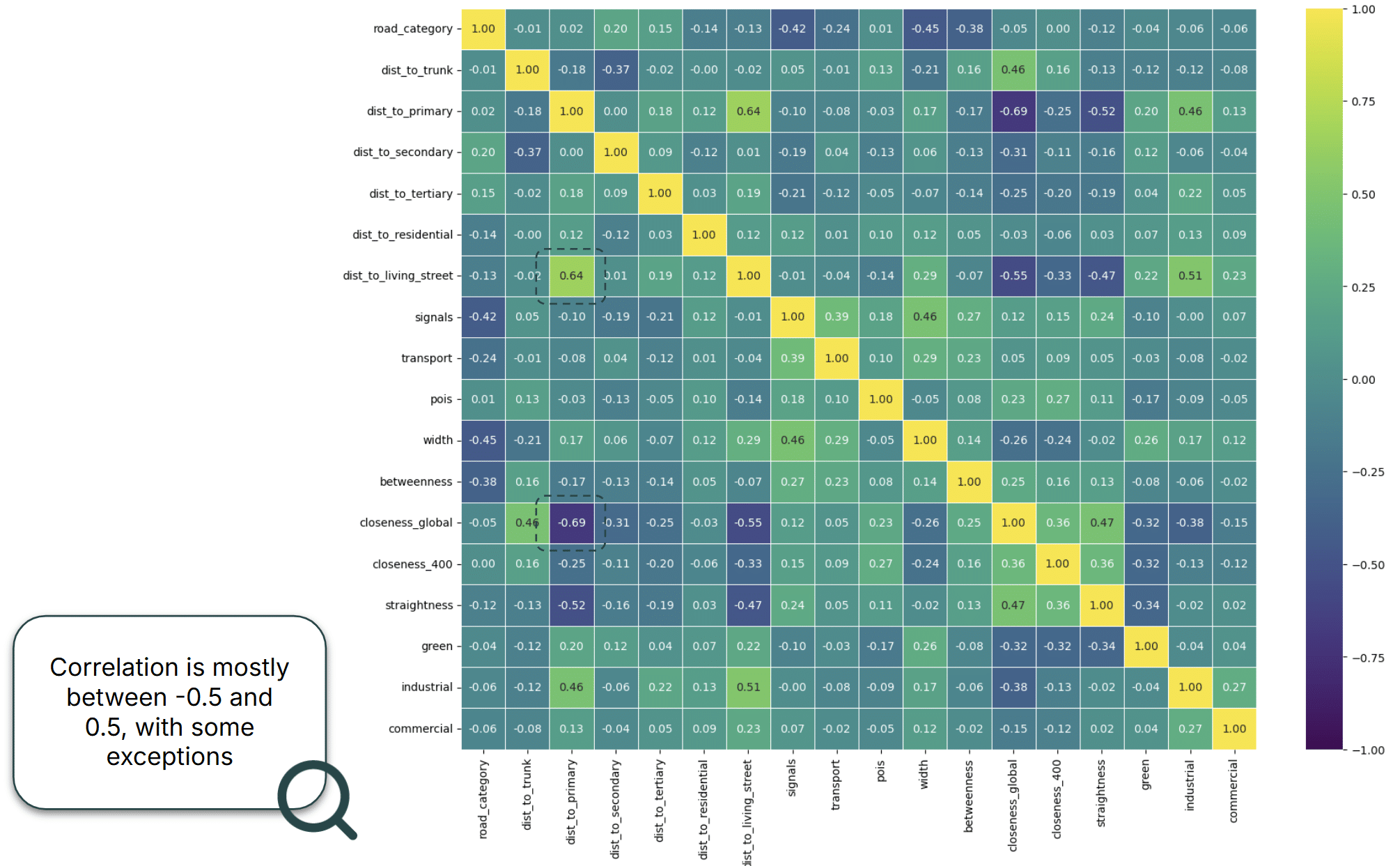
Most feature correlations fell between -0.5 and 0.5, suggesting relatively limited redundancy among predictors.
Is the Feature Space Redundant?
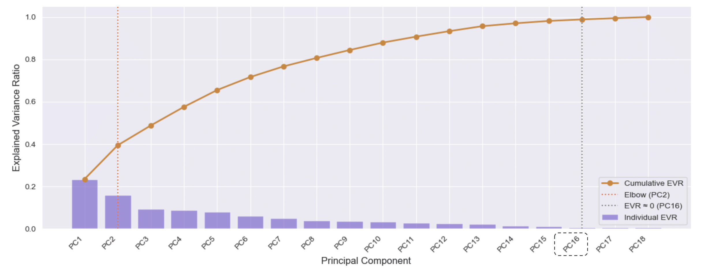
To better understand the structure of the dataset, we performed Principal Component Analysis.
The explained variance curve showed a modest elbow around the second principal component, while cumulative explained variance only began to level off around the sixteenth component.
In other words, the information contained in the dataset is spread across many dimensions rather than concentrated in a handful of variables. This suggests that noise prediction may benefit from models capable of capturing complex interactions among features.
Linear Regression
To investigate how traffic noise prediction varies throughout the day, we trained three regression models—Linear Regression, XGBoost, and Random Forest—separately for daytime, evening, and nighttime conditions.
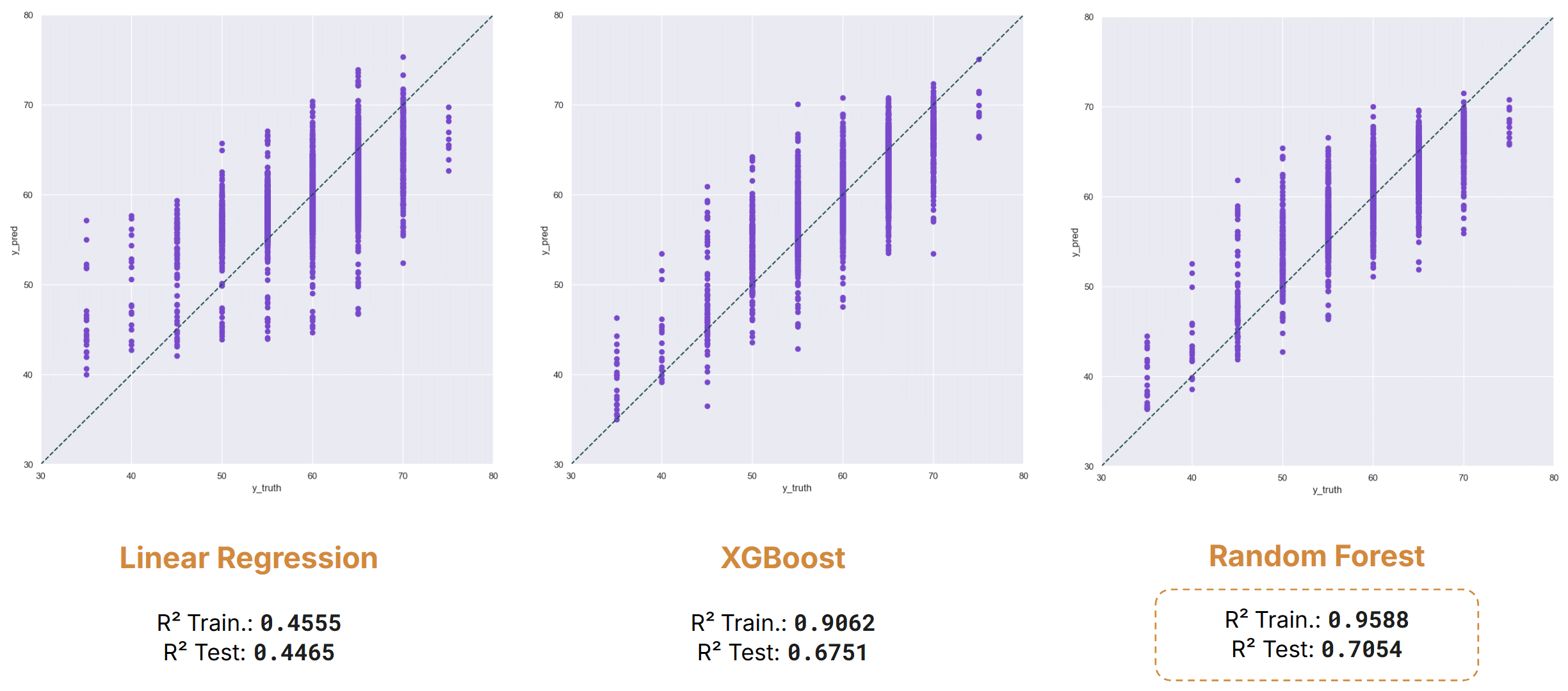
Noise Levels Day
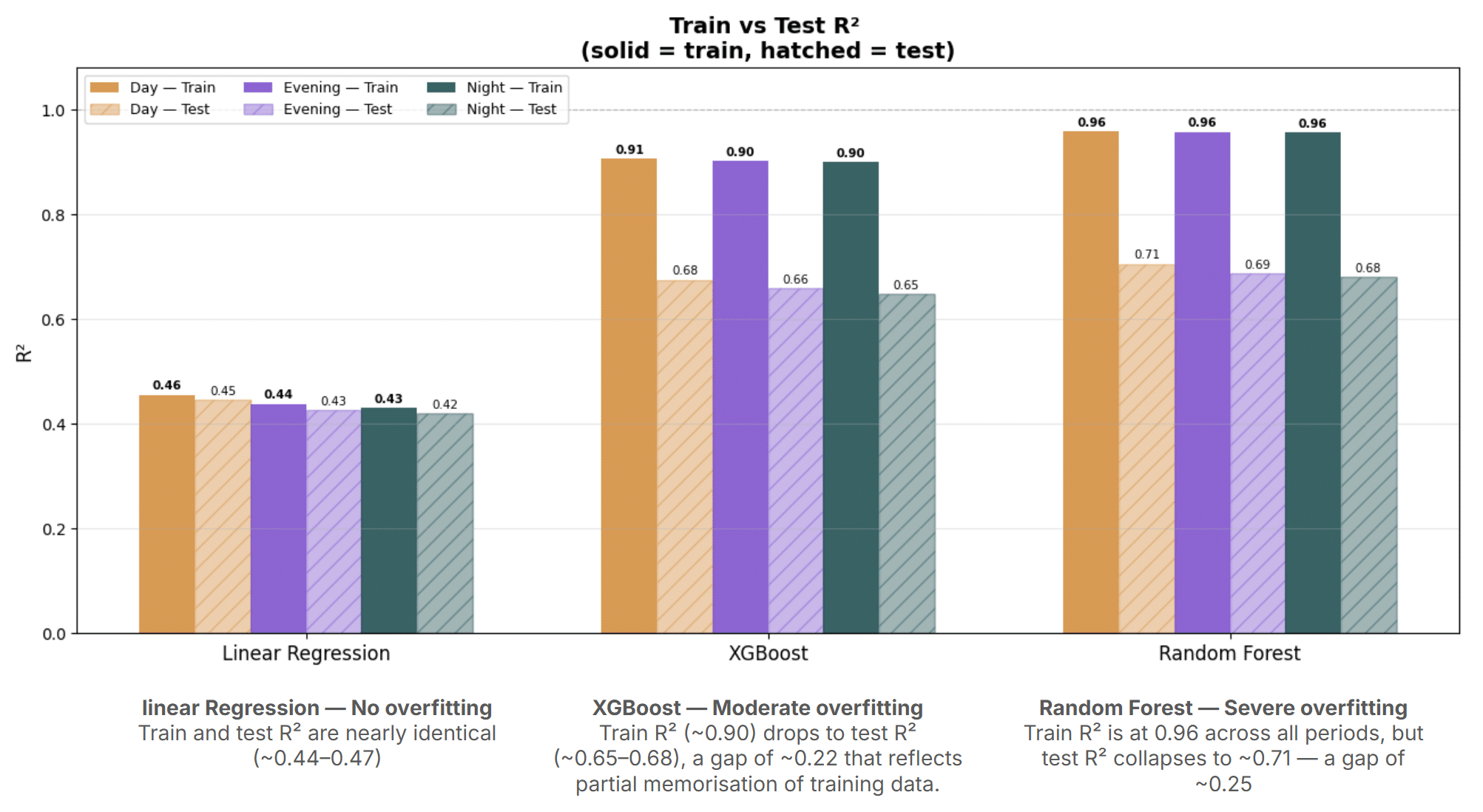
During the daytime period, Linear Regression achieved a test R² score of 0.44, indicating limited ability to capture the underlying relationships in the data. In contrast, the tree-based models performed substantially better, with XGBoost reaching 0.67 and Random Forest achieving 0.70, demonstrating their ability to model more complex, non-linear interactions between features.
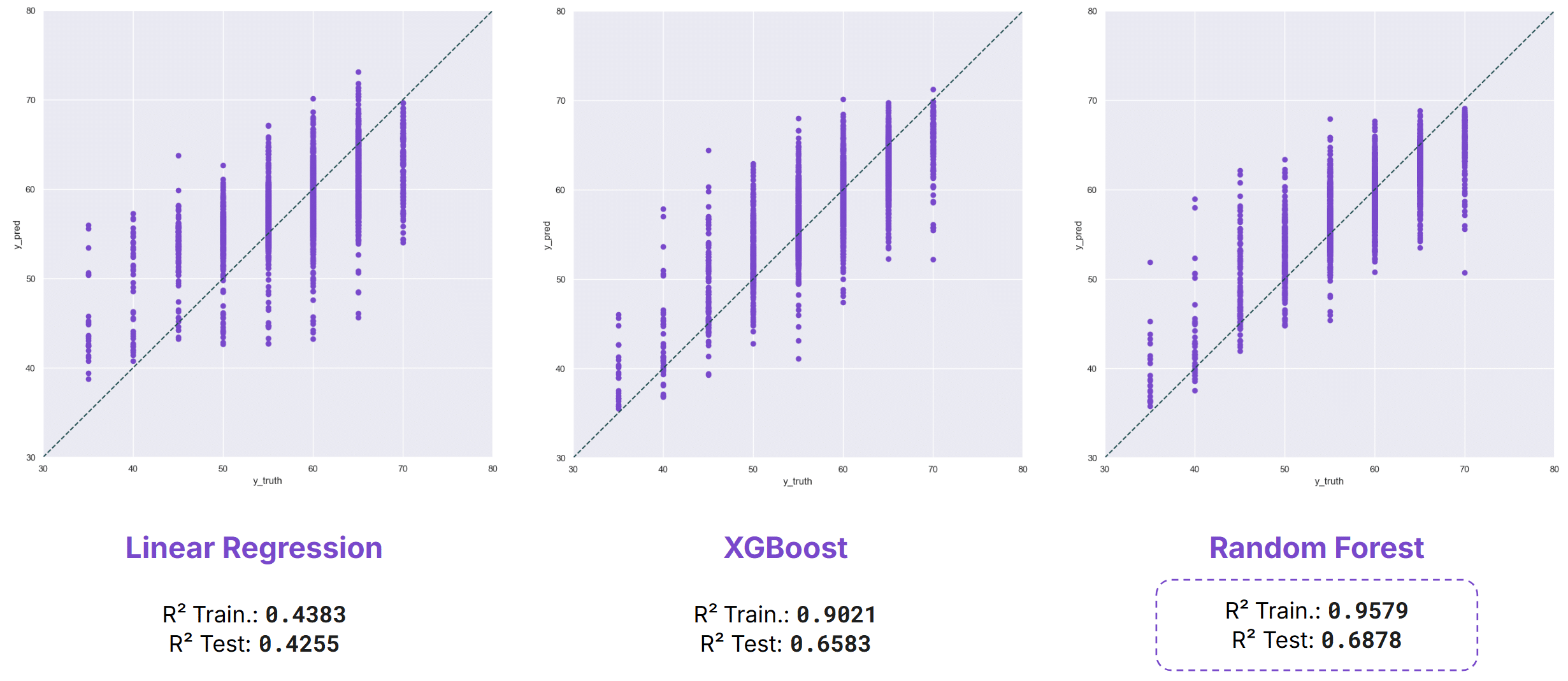
Noise Levels Evening
Model performance during the evening was slightly lower overall. Linear Regression achieved a test R² of 0.42, while XGBoost scored 0.65 and Random Forest scored 0.68. Although the decrease is modest, it suggests that evening traffic patterns may be somewhat less predictable than those observed during daytime hours.
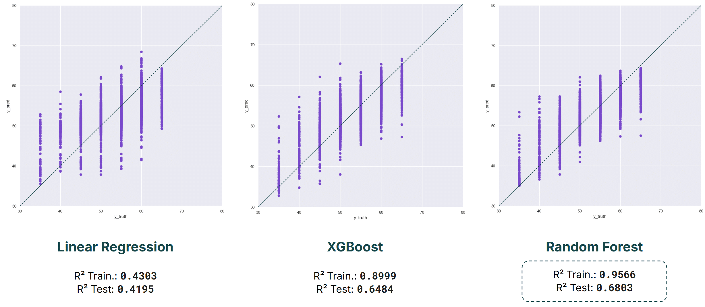
Noise Levels Night
Nighttime results were broadly similar to the evening period. Linear Regression again achieved a test R² of 0.42, while XGBoost and Random Forest obtained scores of 0.65 and 0.68 respectively. This consistency indicates that model performance remains relatively stable outside peak daytime conditions.
Impact of outliers removal
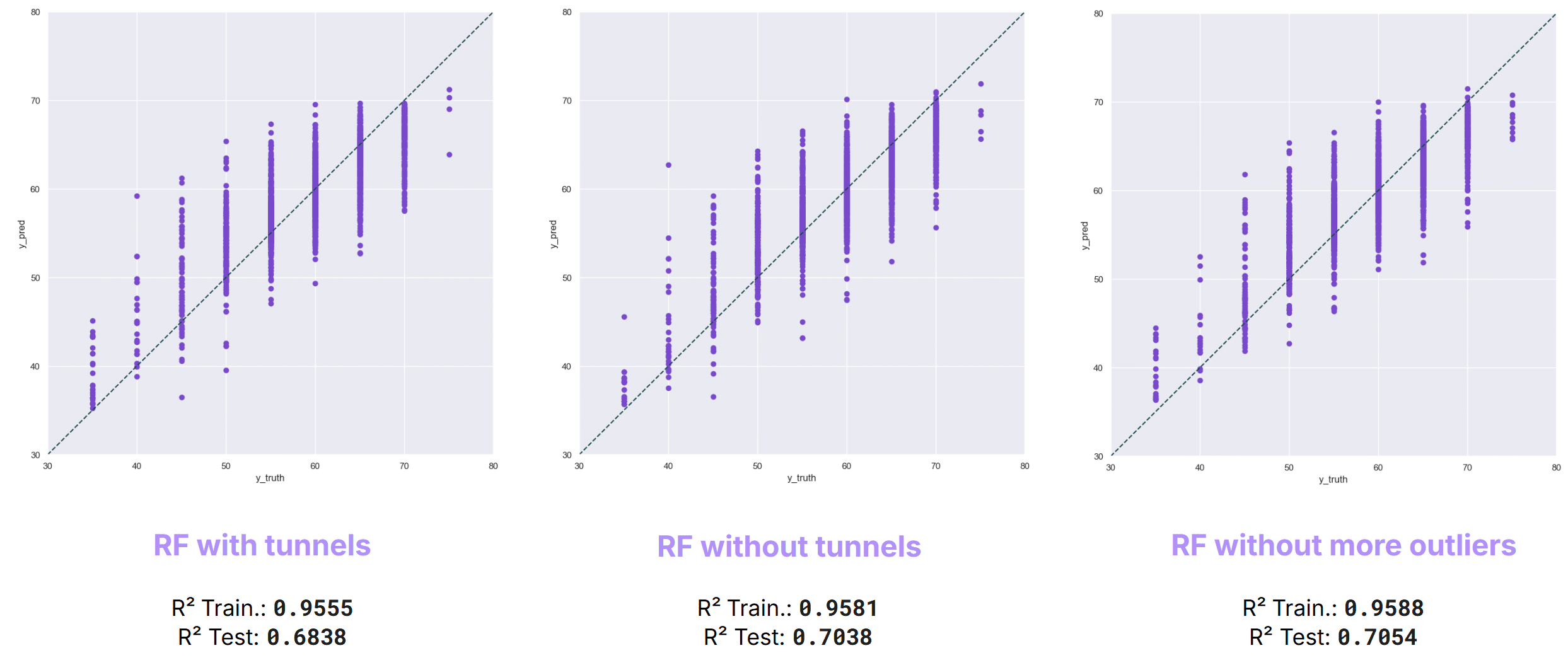
To assess the influence of anomalous road segments, we conducted a comparative analysis using the Random Forest model with and without outlier removal.
Removing tunnel road segments—identified as acoustic outliers due to their atypical noise characteristics—increased the test R² from 0.683 to 0.704, representing the largest single performance improvement observed in this study.
Subsequent removal of additional statistical outliers produced only a marginal increase to 0.705, indicating that tunnel segments were the primary source of noise and model degradation rather than a broader outlier issue within the dataset.
Models Comparison and Generalization
A comparison of training and testing performance reveals a clear degree of overfitting in the tree-based models. Both Random Forest and XGBoost achieved training R² scores exceeding 0.95, yet their test performance dropped to approximately 0.68–0.70.
This gap suggests that while the models successfully captured complex patterns in the training data, some of these patterns did not generalise to unseen examples.
Linear Regression exhibited considerably lower predictive accuracy, maintaining R² values near 0.44 on both training and test datasets across all time periods. While this indicates strong generalisation, it also highlights the model’s inability to capture the complexity of the problem.
Subtractive Ablation Study
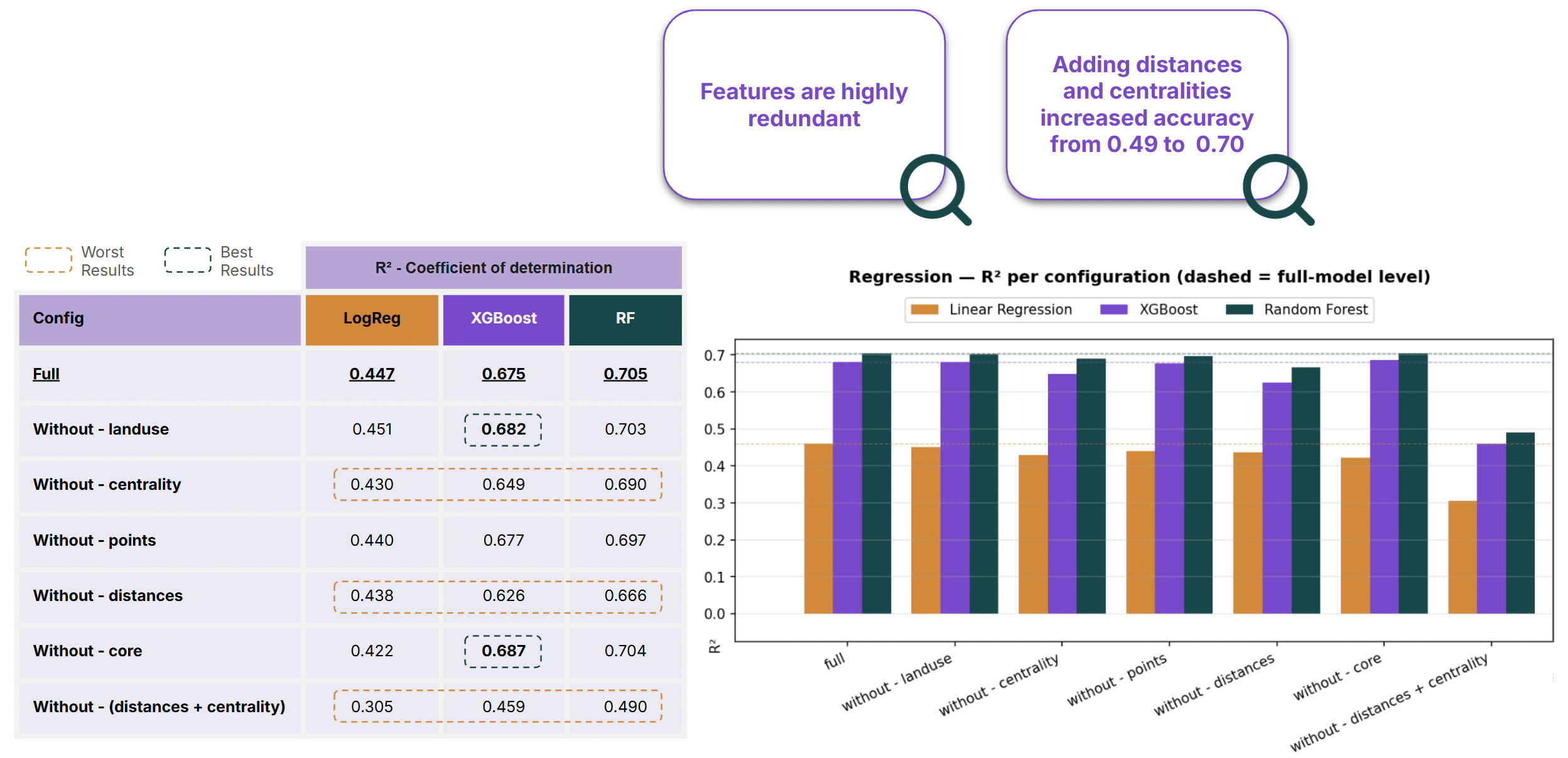
To understand the contribution of each feature group, we performed a subtractive ablation study in which feature categories were removed one at a time and model performance was re-evaluated.
Distance-based metrics and network centrality measures proved to be the most important predictors. Removing either group resulted in the largest decline in model performance, highlighting their central role in explaining urban noise variation.
Conversely, Land Use, Points of Interest, and Core features contributed relatively little to predictive accuracy. In some cases, removing these features slightly improved XGBoost performance, suggesting that they may introduce noise or redundant information.
Independent Feature Analysis
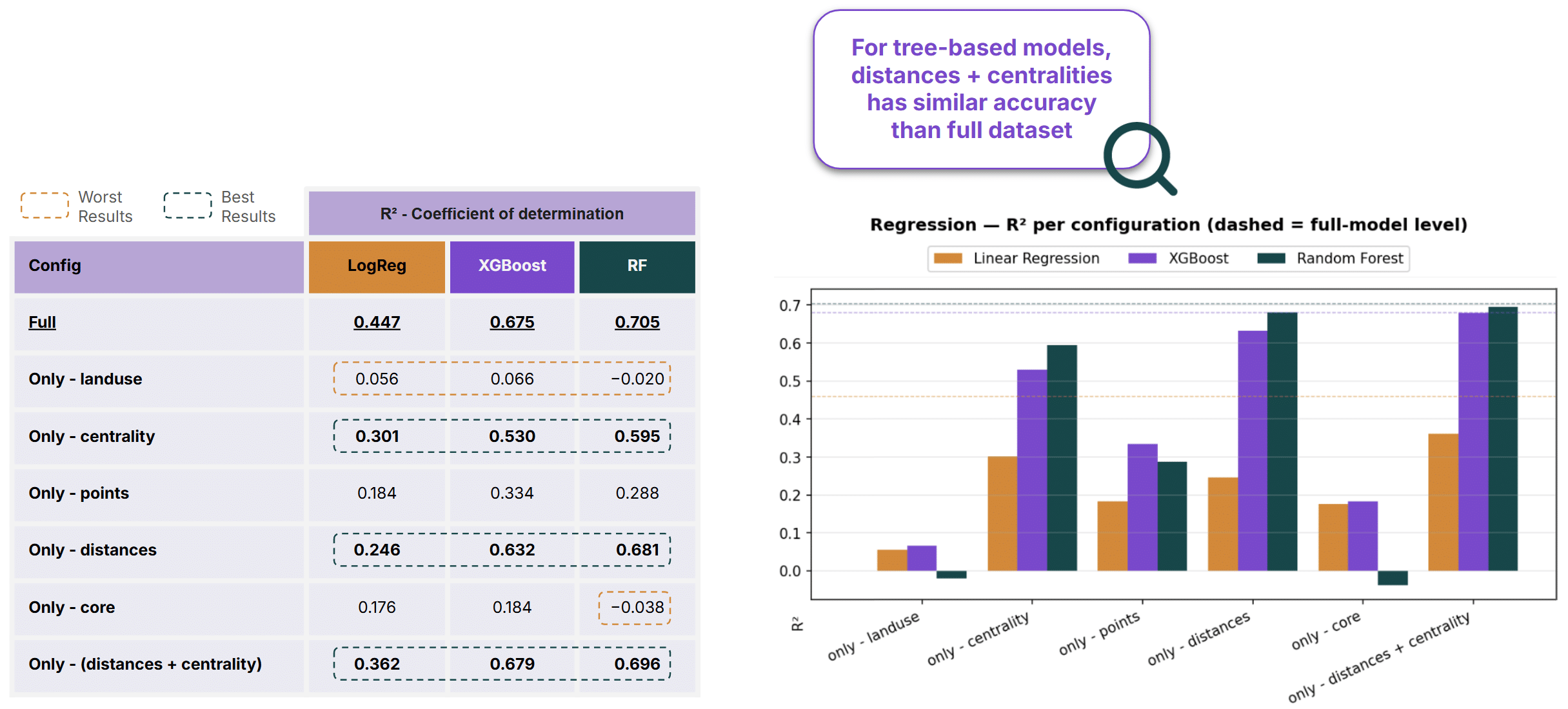
We also conducted an independent feature study to determine how much predictive power each feature group provides on its own.
Using only distance and centrality features, Random Forest achieved an R² score of 0.696, nearly matching the performance of the full feature set. This result indicates that the majority of predictive information is contained within measures describing how roads are connected to the wider transport network.
Consistent with the ablation study, Land Use and Core features contributed the least predictive value. In some cases, their inclusion even reduced Random Forest performance, further supporting the conclusion that these feature groups provide limited useful information for this task.
Artificial Neural Network
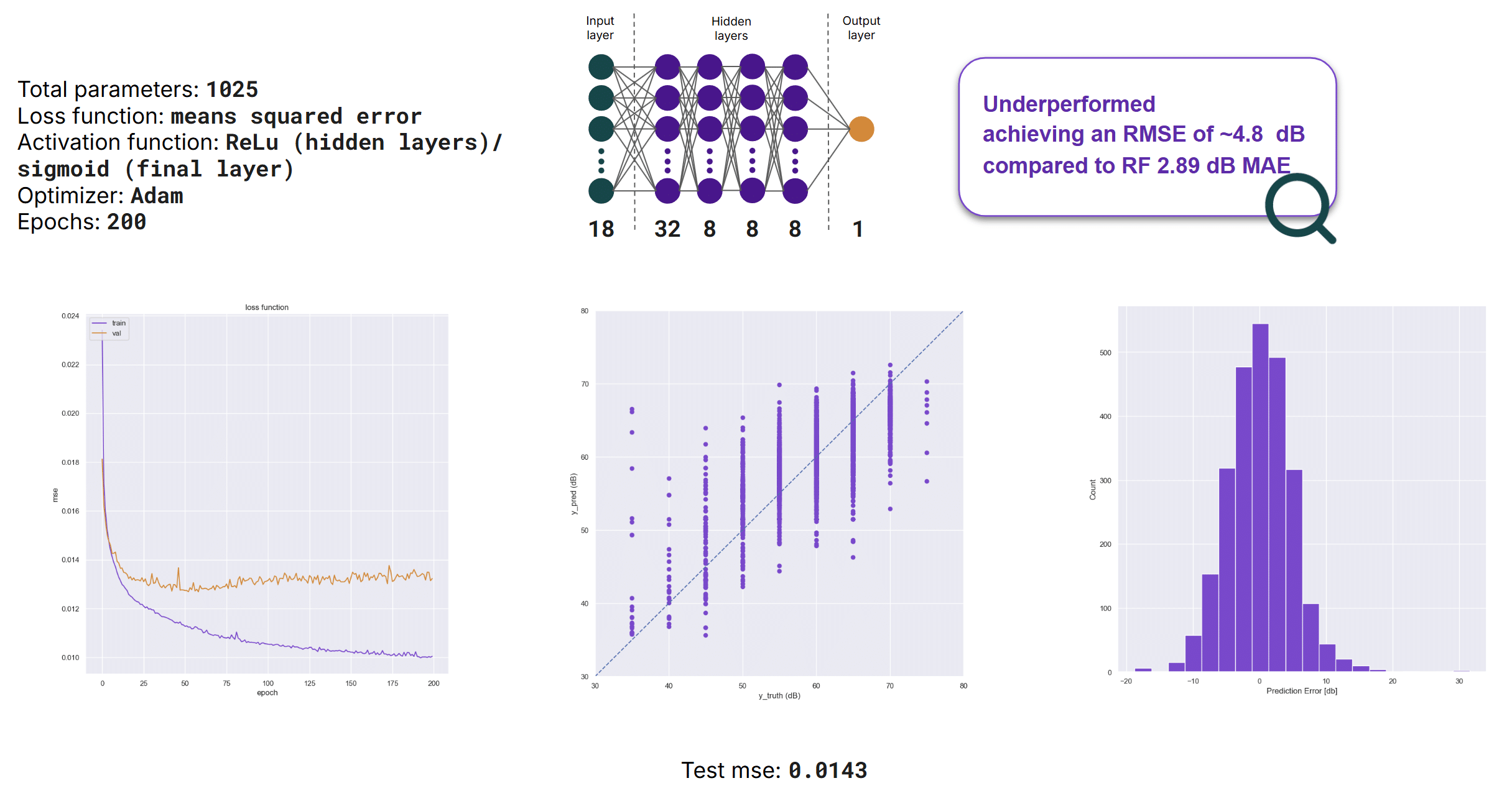
To assess whether deep learning could improve predictive performance, we trained a small Artificial Neural Network (ANN) to predict daytime noise levels.
The network consisted of four hidden layers and 1,025 trainable parameters. Despite this additional complexity, the ANN underperformed compared to the best tree-based models, achieving an RMSE of approximately 4.8 dB, whereas the Random Forest model achieved a mean absolute error (MAE) of 2.89 dB.
These findings suggest that tree-based methods are better suited to this structured tabular dataset, where relationships between variables can be captured effectively without the additional complexity of neural networks.
Model Interpretation with SHAP
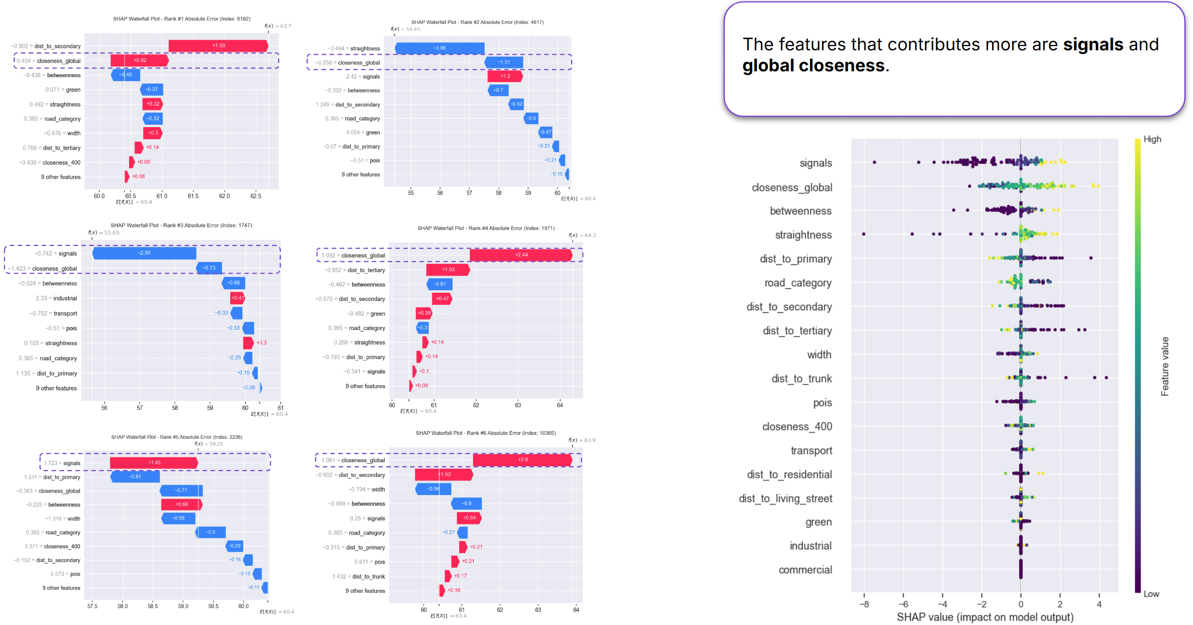
To better understand model predictions and mispredictions, we applied SHAP (SHapley Additive exPlanations) to the Random Forest model.
SHAP decomposes each prediction into contributions from individual features, allowing us to identify which variables drive model behaviour.
The SHAP summary plot strongly reinforces the findings from both ablation studies. Distance-related features—particularly signal proximity and global closeness measures—appear at the top of the importance ranking, indicating the strongest influence on predictions. In contrast, Land Use and Core features appear near the bottom of the ranking, confirming their comparatively limited contribution to model performance.
Classification
Since our regression models couldn’t reach a sufficient level of accuracy, we also explored a classification approach.
We defined 5 different classes with 10 dB ranges, from class 0 for under 40 dB, up to class 4 for over 70 dB. The distribution of the noise levels is roughly Gaussian, with most streets falling into class 3, between 60 and 70 dB. We used the Dummy Classifier, which always predicts Class 3, as our baseline.

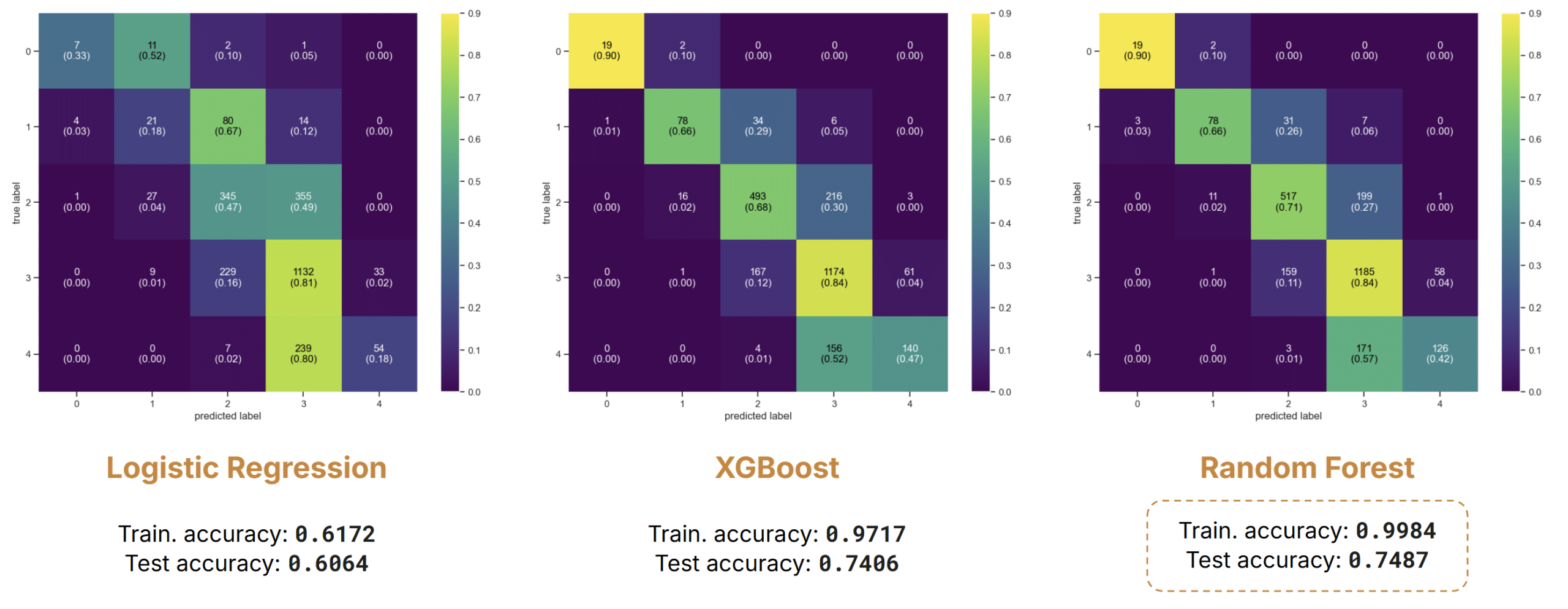
Noise Levels Day
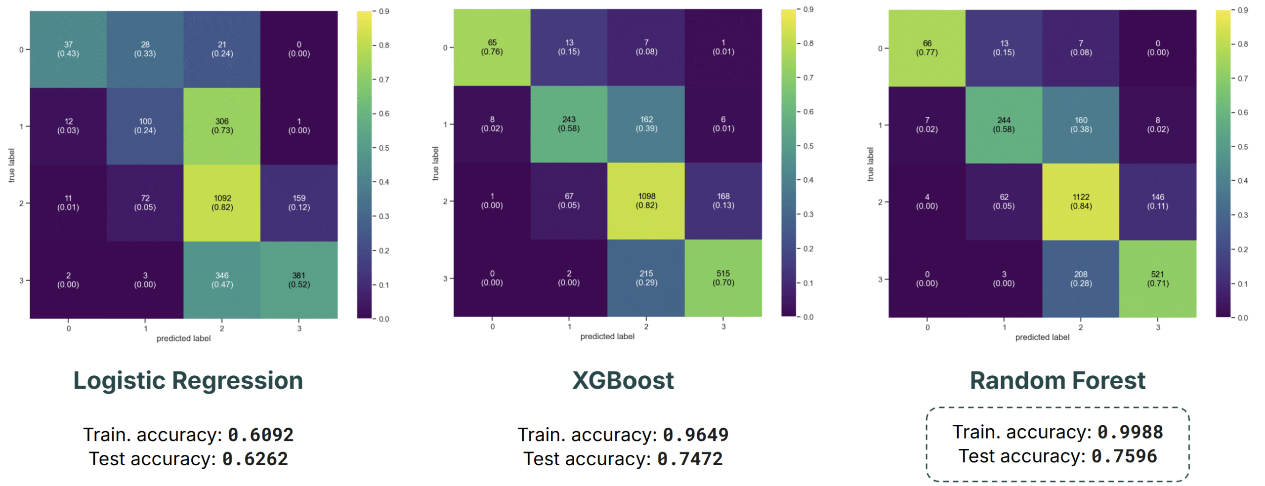
For the daytime noise, XGBoost and Random Forest reached a test accuracy of 74% and 74.9%. While this is a significant improvement, we still see evidence of overfitting, with training accuracy around 99%. As expected, Class 3 has the highest accuracy and most misclassifications underestimate Class 4 as Class 3.
Noise Levels Evening
We repeated the same analysis for evening and night noise levels, obtaining slightly better results in both cases.
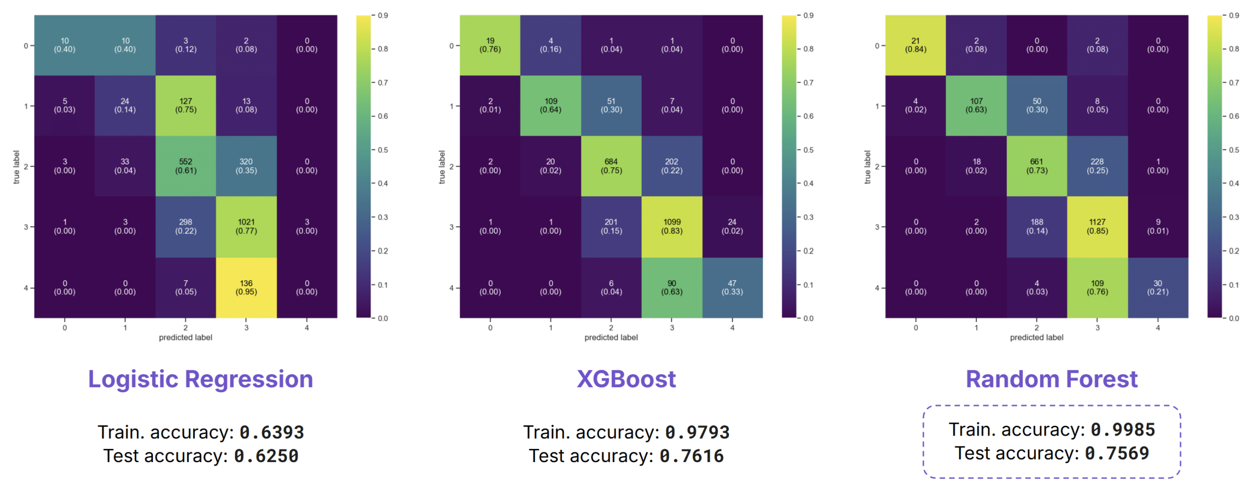
Noise Levels Night
Overall, classification outperforms regression in terms of accuracy, though it’s worth keeping in mind that we’re working with broader, 10 dB-wide bands rather than precise values.
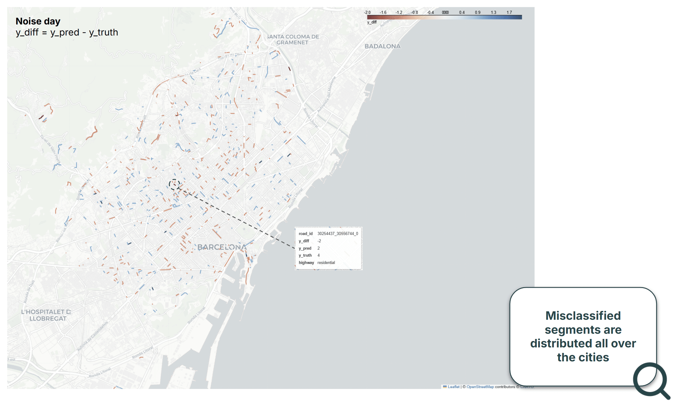
Mapping Results
We mapped the difference between predicted and true labels on an interactive map. From that we can see how misclassified segments are spread across the city, suggesting these errors stem from the inherent limitations of the spatial features rather than from specific location.
Ablation Study
We ran the same ablation study from the regression analysis on our classification models. Adding distances to road categories and centrality measures boosted accuracy from 66% to 75%. Removing centralities alone dropped accuracy to 72.8% for XGBoost and 73.4% for Random Forest, this is important because centrality analyses are particularly time-consuming.
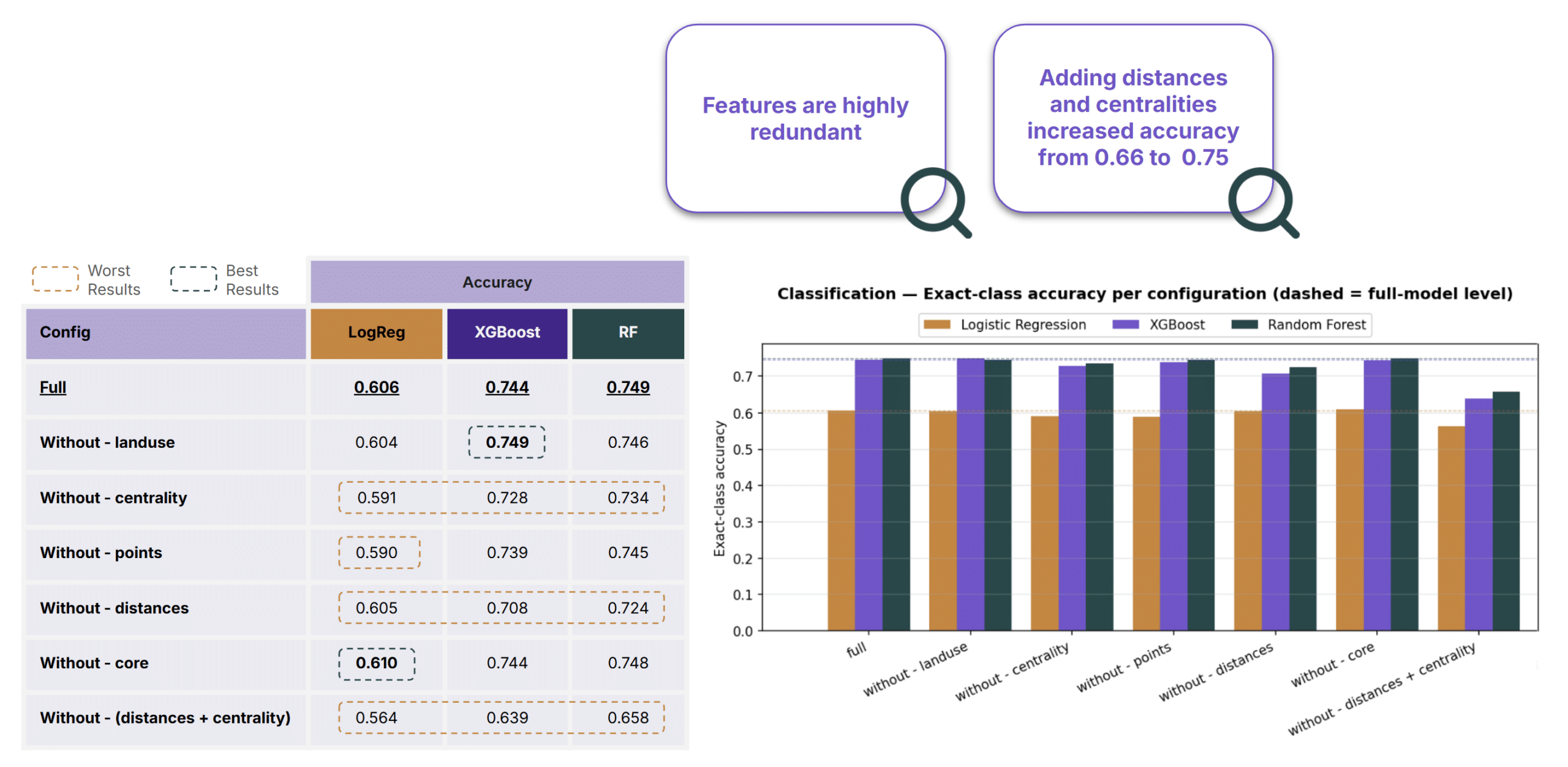
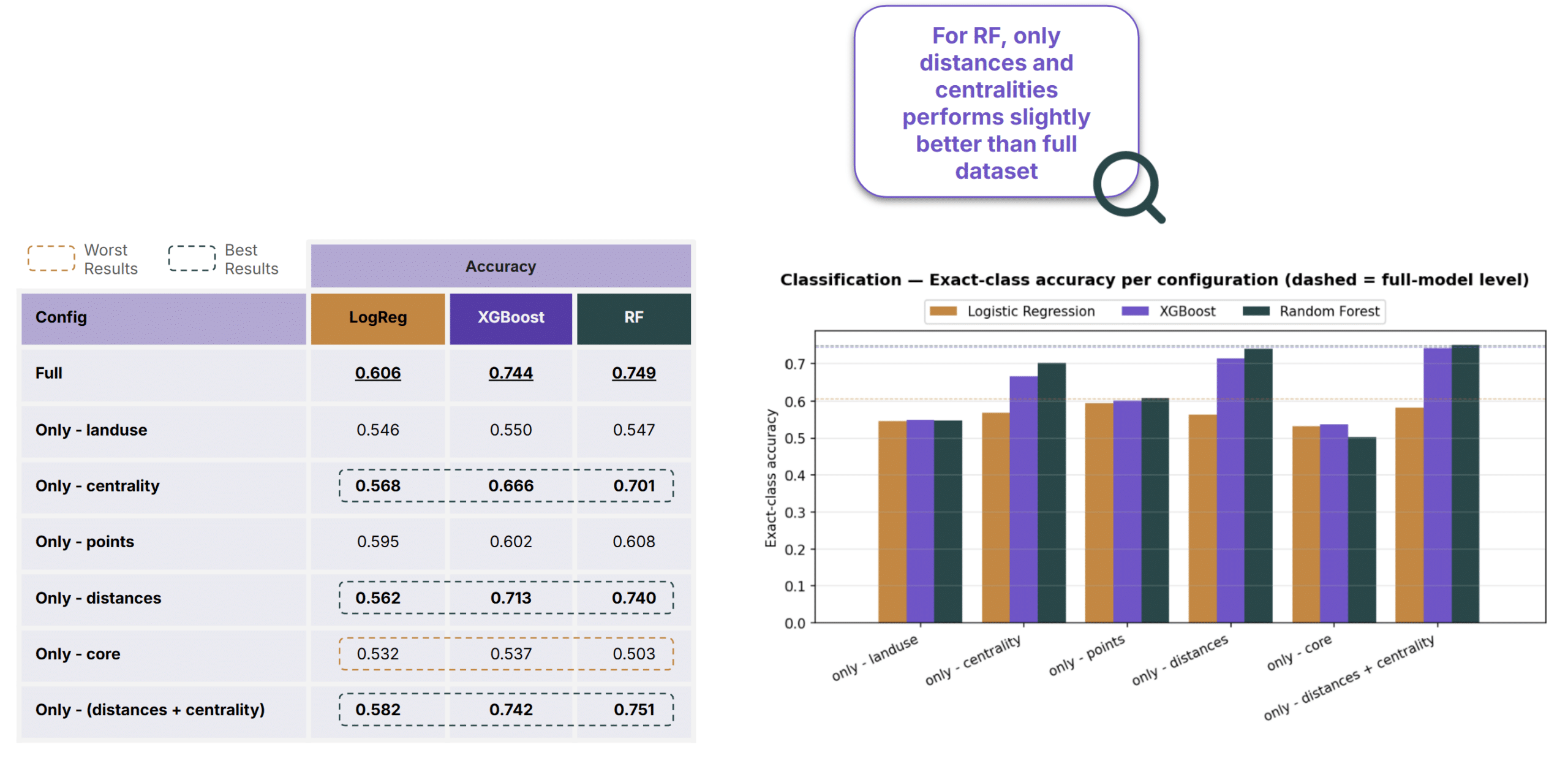
Random Forest, using only distances and centralities performed slightly better than the complete dataset, suggesting some features may be adding noise rather than signal.
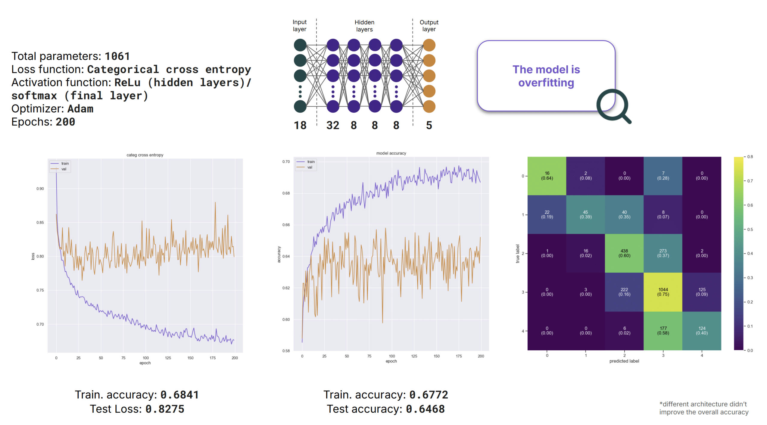
Artificial Neural Network
We also developed an Artificial Neural Network for classification, using the same architecture as our regression Neural Network, but with 5 output layers corresponding to the 5 one hot encoded classes. Again we observed overfitting, and overall performance was lower than XGBoost and Random Forest, reaching 65% accuracy.
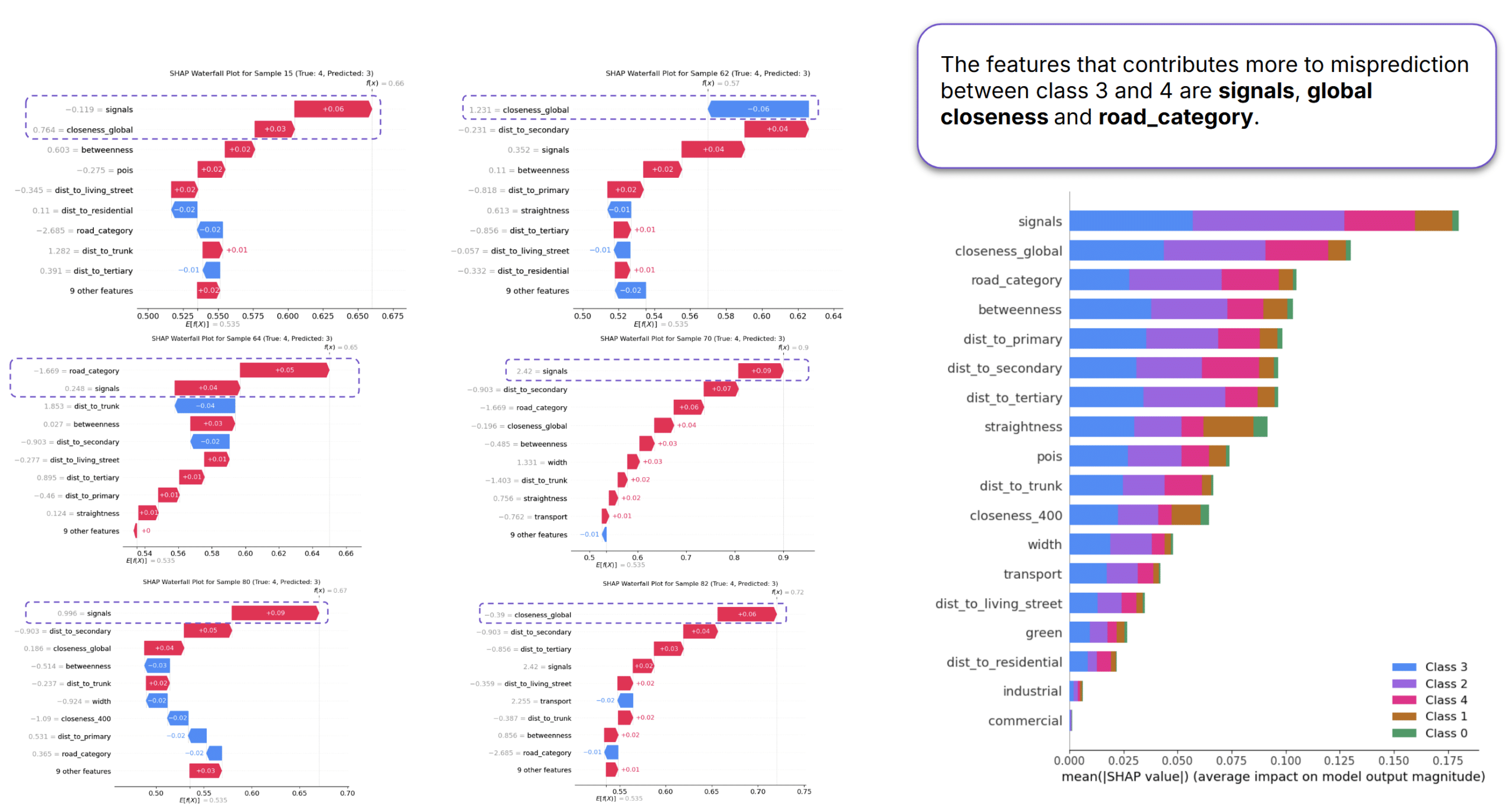
Model Interpretation with SHAP
We ran a SHAP analysis on the Random Forest model to better understand the misclassifications, particularly between Class 3 and Class 4. At the model level, the most influential features were signals, global closeness, and road category.
Deployment
Noise Datasets Sources Comparison
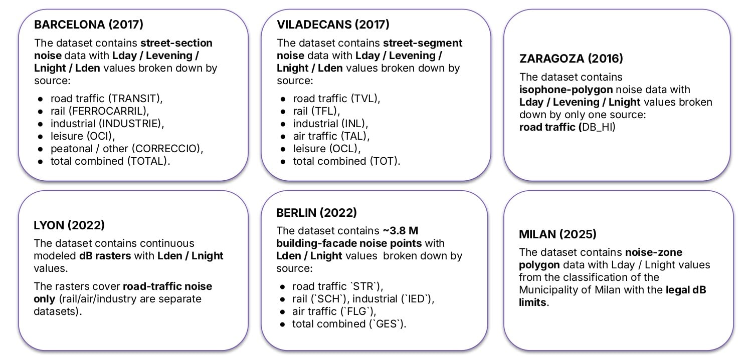
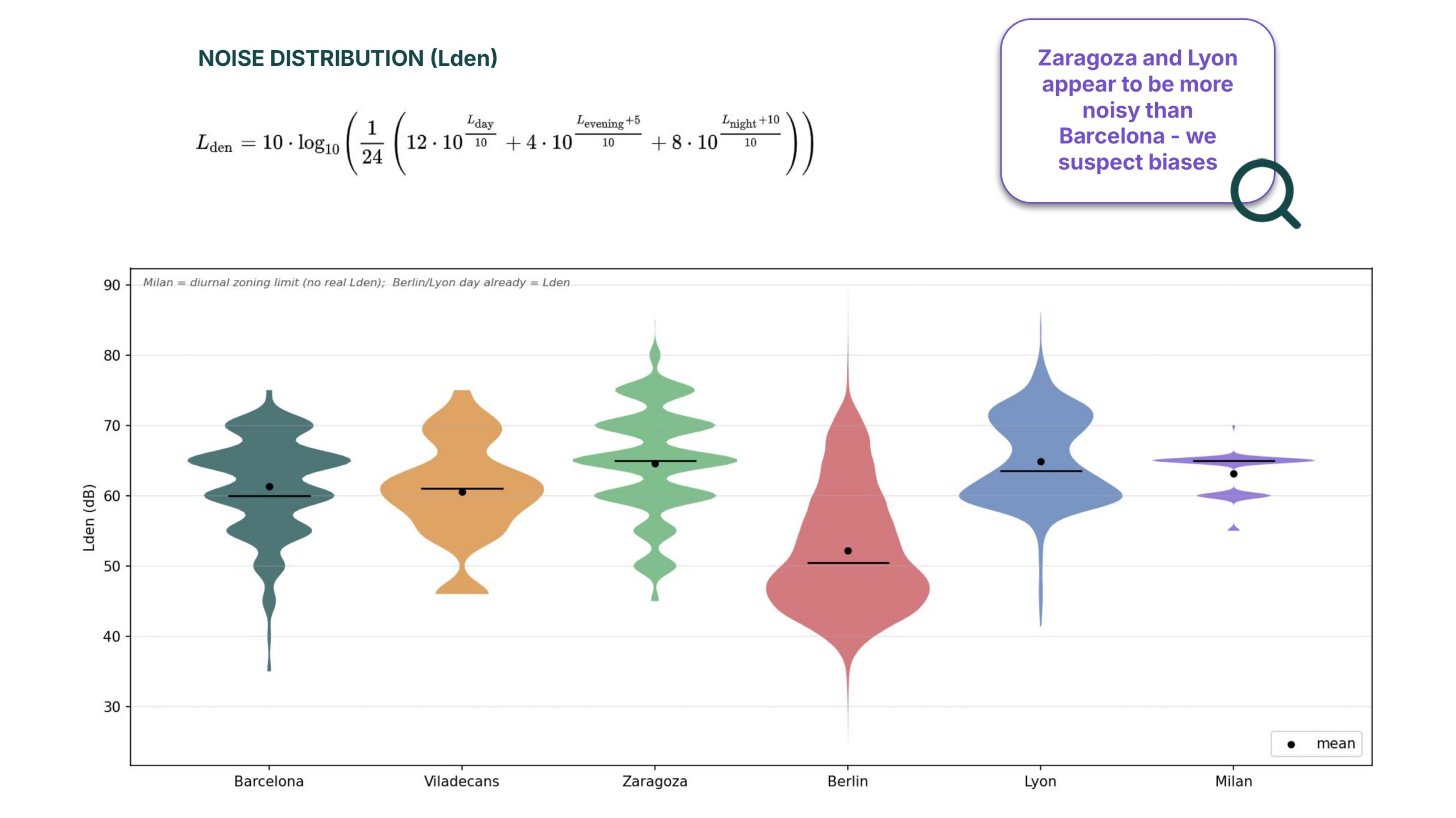
For the deployment of our models, we selected five different cities across Europe. Viladecans is a small Spanish city southwest of Barcelona, featuring a dataset of recorded noise on street segments. Zaragoza’s dataset contains isophone polygons. Meanwhile, Lyon’s data consists of continuous decibel rasters, Berlin provides building-facade noise points, and Milan utilizes noise-zone polygons from the municipality map with legal decibel limits.
All of these datasets natively include Lden values, and most of them account for noise coming from various sources beyond just traffic. Milan was the only city for which we had to approximate the Lden values.
Noise Class & Lden Distribution
Looking at the noise distributions, we can clearly see why our results will change so much between cities. Barcelona is inherently loud, mostly sitting between 60 and 70 decibels. On the other hand, Berlin is much quieter, with nearly half of its streets in the 40-to-50 decibel range.
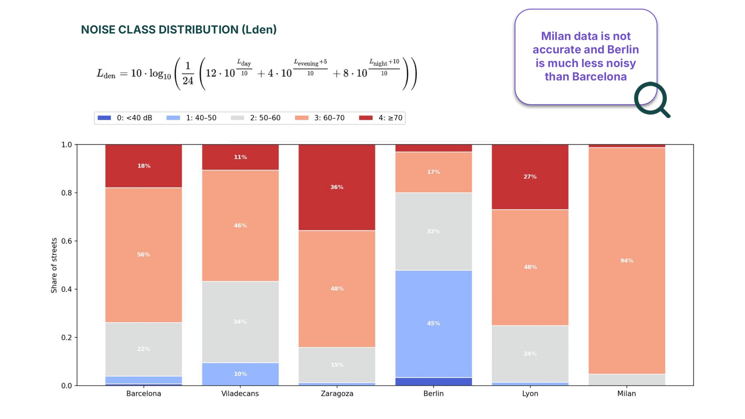
If you look at the violin plots, Milan looks like a flat line. This happens because the data only shows legal limits, so there is no real variance. Meanwhile, Zaragoza and Lyon actually look noisier than Barcelona, which makes us suspect methodological biases. These completely different baselines are the main challenge for our model when we move it to another city.”
Regression Models Performance
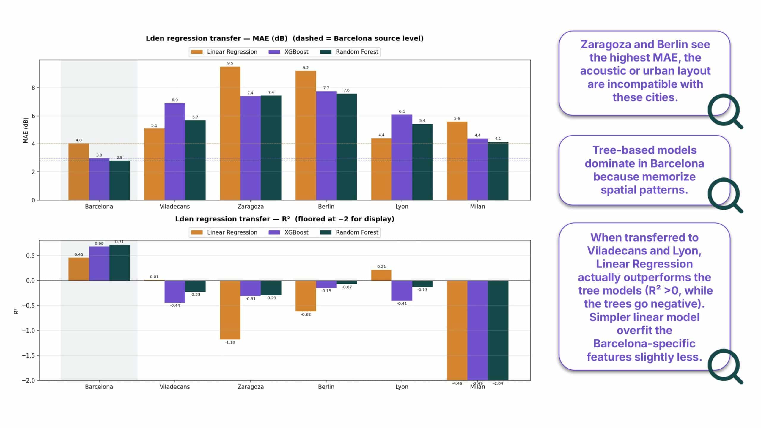
Analyzing regression performance, tree-based models like Random Forest dominate in our training city because they are good at memorizing local spatial patterns. However, they struggle out-of-domain.
The Mean Absolute Error spikes in Zaragoza and Berlin because their urban layouts are fundamentally incompatible with Barcelona’s. Interestingly, when we transfer to Viladecans and Lyon, simpler Linear Regression actually outperforms the tree models. Because it’s less flexible, it doesn’t overfit to Barcelona’s specific geometry and transfers more cleanly.
Classification Accuracy
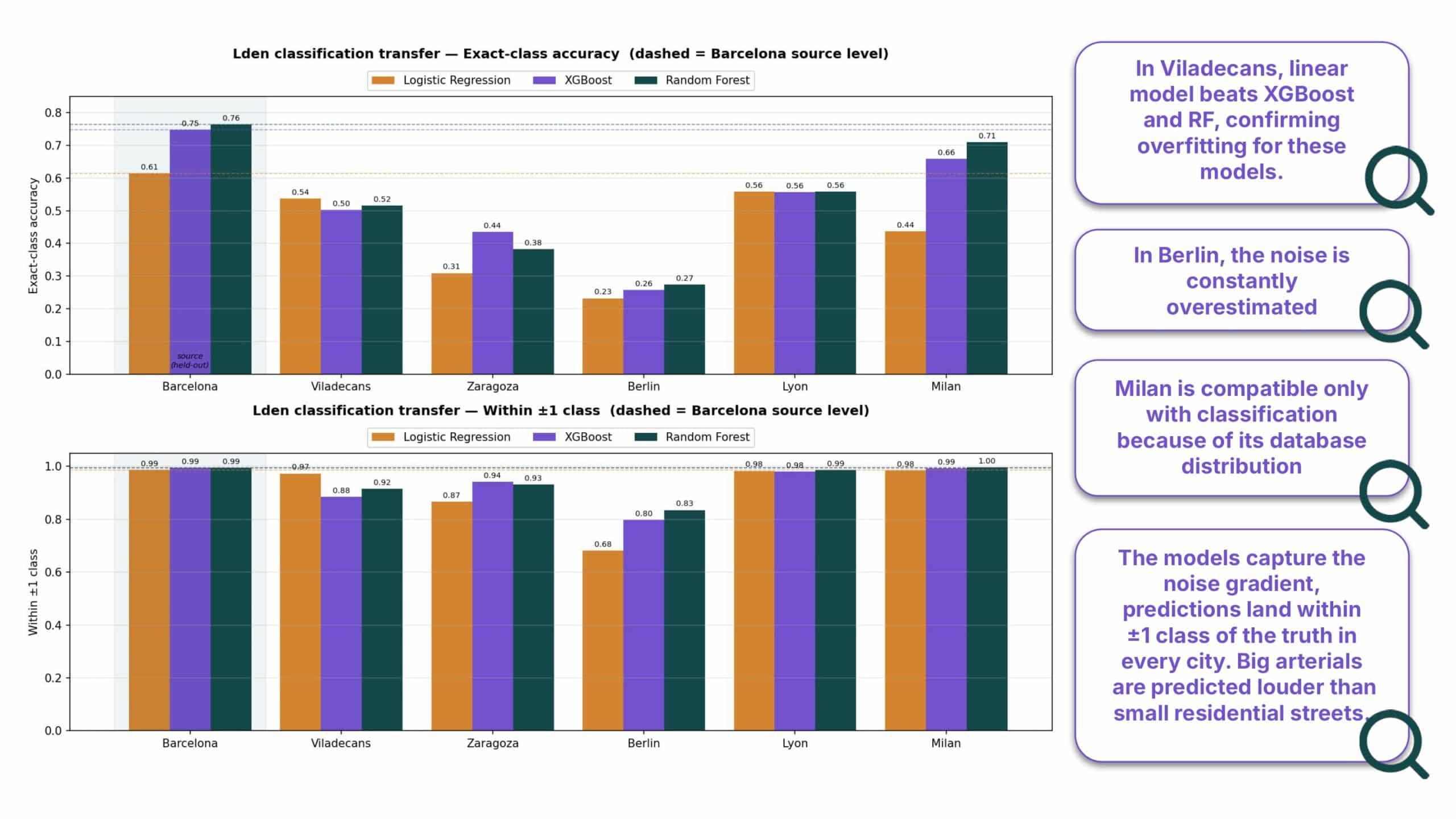
Evaluating classification, again, in Viladecans, the linear model beats out XGBoost and Random Forest, confirming our suspicions about overfitting. In Berlin, our models consistently overestimated the noise levels.
While exact-class accuracy drops significantly, the within-plus-or-minus-one class accuracy shows good results. This is the main success of the deployment. It proves our models capture the underlying spatial noise gradient everywhere. They consistently recognize that a massive arterial road is louder than a tiny residential alley, even if the absolute baseline decibel level has shifted.
Interpretation
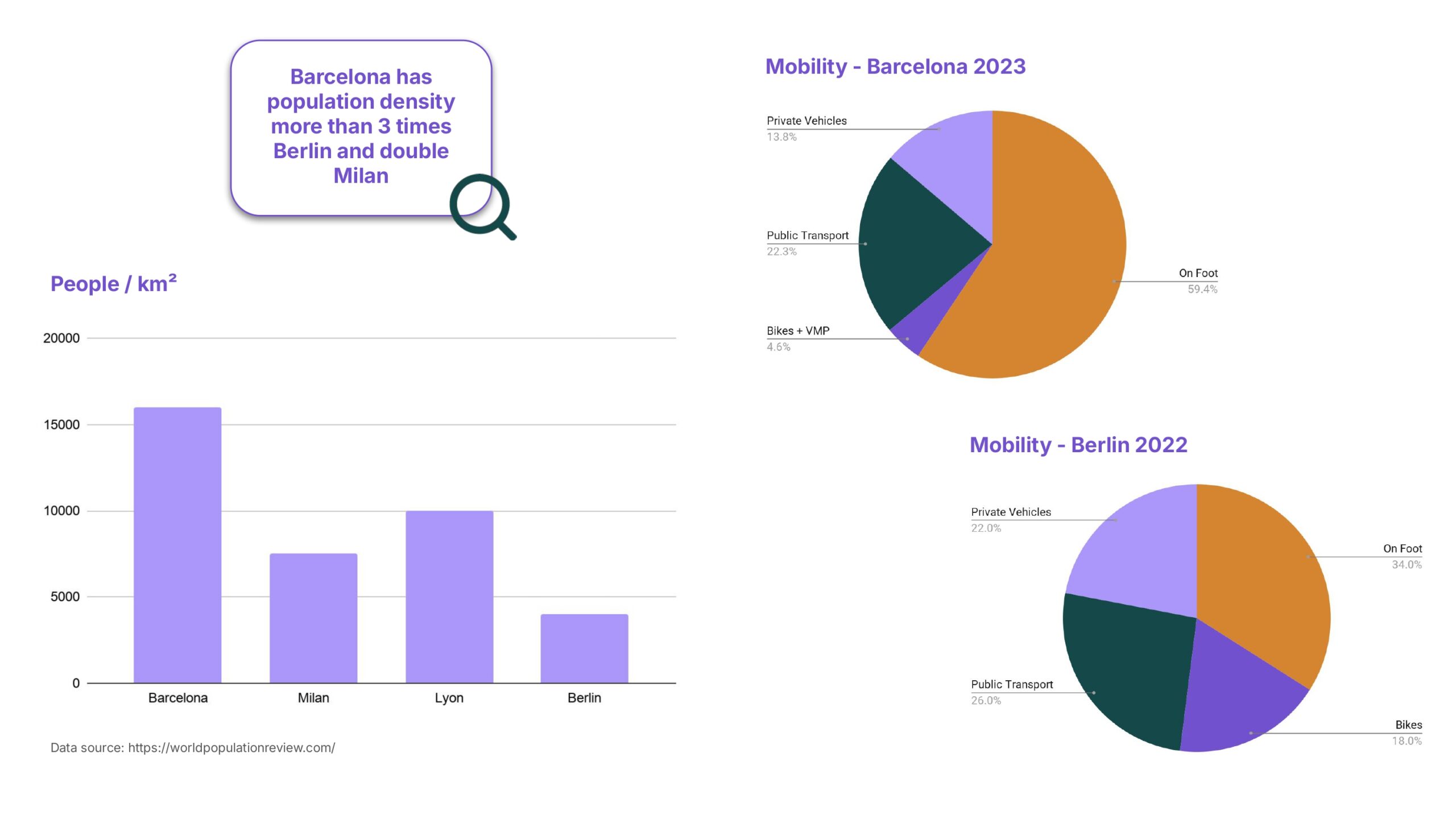
Noise isn’t just about street geometry; it’s about people. As you can see, Barcelona has a population density more than three times that of Berlin and double that of Milan.
Furthermore, mobility patterns are drastically different. In Barcelona, almost 60% of mobility is on foot, compared to just 34% in Berlin, which has a much higher share of private vehicle usage. These demographic and cultural factors inherently dictate urban noise, making raw spatial transferability incredibly difficult without local context.
Conclusions
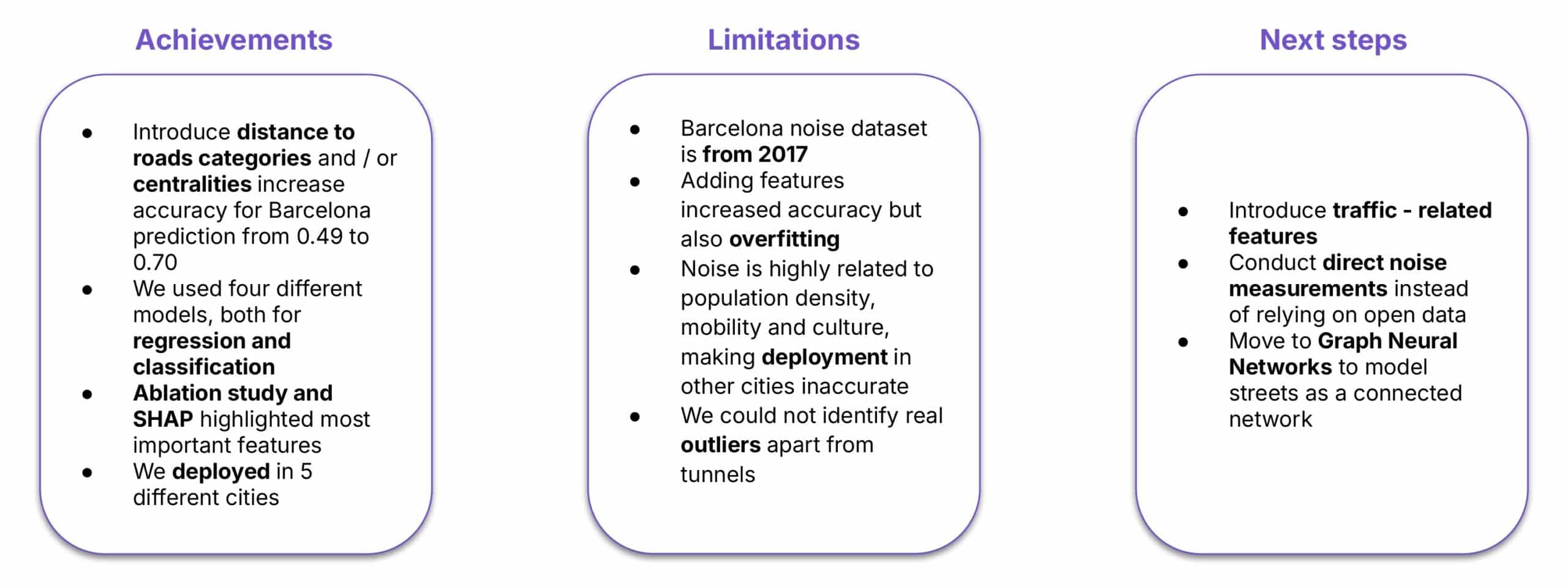
Starting from achievements, we raised our prediction accuracy in Barcelona from 49% to 70% by adding features like distance to roads and street centrality. We built and compared four different models, used SHAP values to find the most important featurs, and successfully tested our models in five other European cities.
Of course, we have some limitations. Our Barcelona data is from 2017. Also, while our new features improved accuracy, they also caused some overfitting. As we just saw, noise depends heavily on population density and how people move, which makes it hard to use the model in new cities without changes. Finally, finding real outliers was very difficult, except for tunnels.
Looking ahead, our next steps to develop this project further are clear. Add live traffic features, collect own direct noise measurements instead of relying on different open datasets. Ultimately, try transitioning to Graph Neural Networks, which will help us model streets as the connected, living networks they really are.
Bibliography
Traffic noise assessment in urban Bulgaria using explainable machine learning (2025)
Interpretable machine learning of urban noise levels from street-scale morphology and functionality (2026)
